ダブルEMAゴールデンクロスとデスクロス追跡戦略

概要
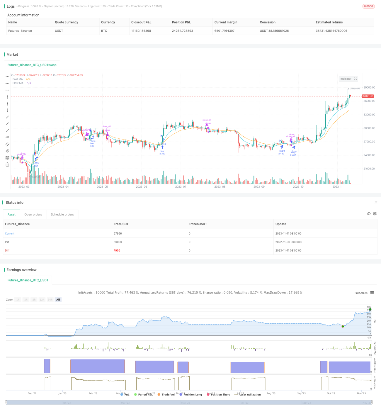
この戦略は,快線EMAと慢線EMAを計算し,両者の大きさの関係を比較することによって,双EMAの金叉と死叉の取引信号を実現し,トレンド追跡戦略の1つである. 快線が慢線を横切るときに買い信号を生成し,快線が慢線を横切るときに売り信号を生成し,簡単なトレンド追跡戦略を実現する.
戦略原則
この戦略の核心的な論理は以下の部分から構成されています.
-
速線EMAと遅線EMAを計算する: fastInputの速線EMAとslowInputの遅線EMAの長さを ta.ema (()) 関数で計算する.
-
回測時間範囲を設定する:useDateFilterのパラメータで回測時間,backtestStartDate,backtestEndDateの開始と終了時間を設定する.
-
取引シグナルを生成:ta.crossover ((() とta.crossunder ((() の関数で,快線EMAと遅線EMAの大きさの関係を比較し,快線上での遅線通過時に買取シグナルを生成し,快線下での遅線通過時に売り出シグナルを生成する.
-
処理時間枠外の注文: 回測時間枠外で未処理の注文をキャンセルし,すべてのポジションを平らにする.
-
移動平均を描画:グラフに速線EMAと遅線EMAの移動平均を描画する.
戦略的優位性
これは非常に単純なトレンド追跡戦略で,以下の利点があります.
-
戦略の論理はシンプルで,理解し,実行しやすい.
-
EMAは価格データを平らにしており,取引の騒音を減らすことができます.
-
EMA周期パラメータをカスタマイズし,異なる市場環境に対応する.
-
柔軟に設定できる反射時間帯で,特定の時間帯に合わせてテストを行う.
-
入場・出場条件を最適化し,他の指標と組み合わせて使用する.
リスク分析
この戦略にはいくつかのリスクがあります.
-
双重EMAの戦略は,市場変化に柔軟に対応できないほど粗略である.
-
取引の頻度や重複の危険性がある
-
EMAパラメータの設定を間違えた場合,取引シグナルのエラーが発生する可能性があります.
-
返信時間帯の不合理な範囲は,過適合を引き起こす可能性があります.
-
強制撤回と損失の危険性がある
パラメータの最適化,適切なフィルター波動,停止の設定などの方法でリスクを制御できます.
最適化の方向
この戦略は以下の点で最適化できます.
-
EMA周期パラメータを最適化し,最適なパラメータ組み合わせを選択する.
-
フィルタリングを追加し,不要な取引を回避します.
-
単一損失を抑えるためのストップ・ロース戦略を導入する.
-
トレンド,波動率などのフィルターと組み合わせて,取引の頻度を減らす.
-
異なる品種の契約をテストし,最適の戦略を適用する対象を探します.
-
スライドポイント,手数料などのコスト管理により,反測はよりリアルになります.
要約する
この戦略は,全体的に非常に単純な双EMA金叉死叉戦略であり,論理が明確で分かりやすく,高速でゆっくりとした線EMA比較によって取引信号を生成する.この戦略の優点は,実行が簡単である,しかし,頻繁な取引,過剰最適化を引き起こす可能性などのいくつかの問題もあります.次のステップは,パラメータ最適化,リスク管理などの面で改善され,戦略をより堅牢に実用的にすることができます.
/*backtest
start: 2022-11-06 00:00:00
end: 2023-11-12 00:00:00
period: 1d
basePeriod: 1h
exchanges: [{"eid":"Futures_Binance","currency":"BTC_USDT"}]
*/


//@version=5
strategy("MollyETF_EMA_Crossover", overlay = true, initial_capital = 100000, default_qty_value=100, default_qty_type=strategy.percent_of_equity)
- 1