極性フラクタル効率(PFE)取引戦略

概要
極性フラクタル効率(Polarized Fractal Efficiency, PFE)取引戦略は、フラクタル幾何学とカオス理論の概念を応用し、価格変動の効率性を測定します。価格変動が線形で効率的であるほど、2点間の距離は短くなり、価格変動の効率性は高まります。
戦略原理
PFE取引戦略の中心指標は極性フラクタル効率(PFE)です。この指標は以下の式に基づいて計算されます。
PFE = sqrt(pow(close - close[Length], 2) + 100)
ここで、Lengthはルックバック期間であり、このパラメータは入力によって設定されます。PFEは実際には、Length期間における価格変動の「長さ」を測定するものであり、ユークリッド距離(直線距離)を用いて近似的に測定します。
価格変動の効率性を評価するためには、比較の基準が必要です。この基準は、Length期間において価格が実際の順序で連結された経路の長さであり、C2C(Close to Close)と呼ばれ、以下の式で計算されます。
C2C = sum(sqrt(pow((close - close[1]), 2) + 1), Length)
これにより、価格変動のフラクタル効率xFracEffを計算できます。
xFracEff = iff(close - close[Length] > 0, round((PFE / C2C) * 100) , round(-(PFE / C2C) * 100))
価格が上昇した場合は正の値、下落した場合は負の値となります。絶対値が大きいほど、変動の効率が低いことを示します。
取引シグナルを生成するために、xFracEffの指数移動平均であるxEMAを計算します。また、買い・売りのチャネルを設定します。
            xEMA = ema(xFracEff, LengthEMA)

BuyBand = input(50)
SellBand = input(-50)
xEMAがBuyBandを上方にクロスした場合に買いシグナル、xEMAがSellBandを下方にクロスした場合に売りシグナルを生成します。
優位性分析
PFE取引戦略には以下の優位性があります。
- 独自のフラクタル幾何学とカオス理論の手法を応用し、別の角度から価格変動の効率性を測定する。
- カーブフィッティングなど、従来のテクニカル指標にありがちな問題を回避する。
- パラメータを調整することで、様々な市場環境に適した設定を見つけることができる。
- 取引ルールがシンプルかつ明確で、実装が容易である。
リスク分析
PFE取引戦略には以下のリスクも存在します。
- 他の指標戦略と同様に、パラメータの最適化が困難であり、過剰最適化に陥りやすい。
- 市場が激しく変動する場合、売買シグナルが信頼できない可能性がある。
- 極端な値、例えば価格が突然ギャップを生じる場合の処理には注意が必要である。
- 一定のタイムラグが生じ、シグナルが発生した時点で最適なエントリーポイントを逃している可能性がある。
最適化の方向性
PFE取引戦略は、以下の観点から最適化が可能です。
- 異なるLengthパラメータの組み合わせを試し、最適なバランス点を見つける。
- 売買チャネルのパラメータを最適化し、誤った取引の確率を低減する。
- ストップロス機構を追加し、1回の損失を抑制する。
- 他の指標と組み合わせ、シグナルの品質を向上させる。
- パラメータを動的に調整し、市場環境の変化に適応する。
まとめ
PFE取引戦略は、フラクタル幾何学とカオス理論の視点に基づき、価格変動の効率性を測定する新しい手法を提案します。従来のテクニカル指標と比較して、この手法には独自の利点がありますが、同時にある程度のタイムラグ、パラメータ最適化、シグナル品質の問題にも直面します。継続的なテストと最適化を通じて、PFE戦略は信頼性の高い定量取引戦略の選択肢となる可能性があります。
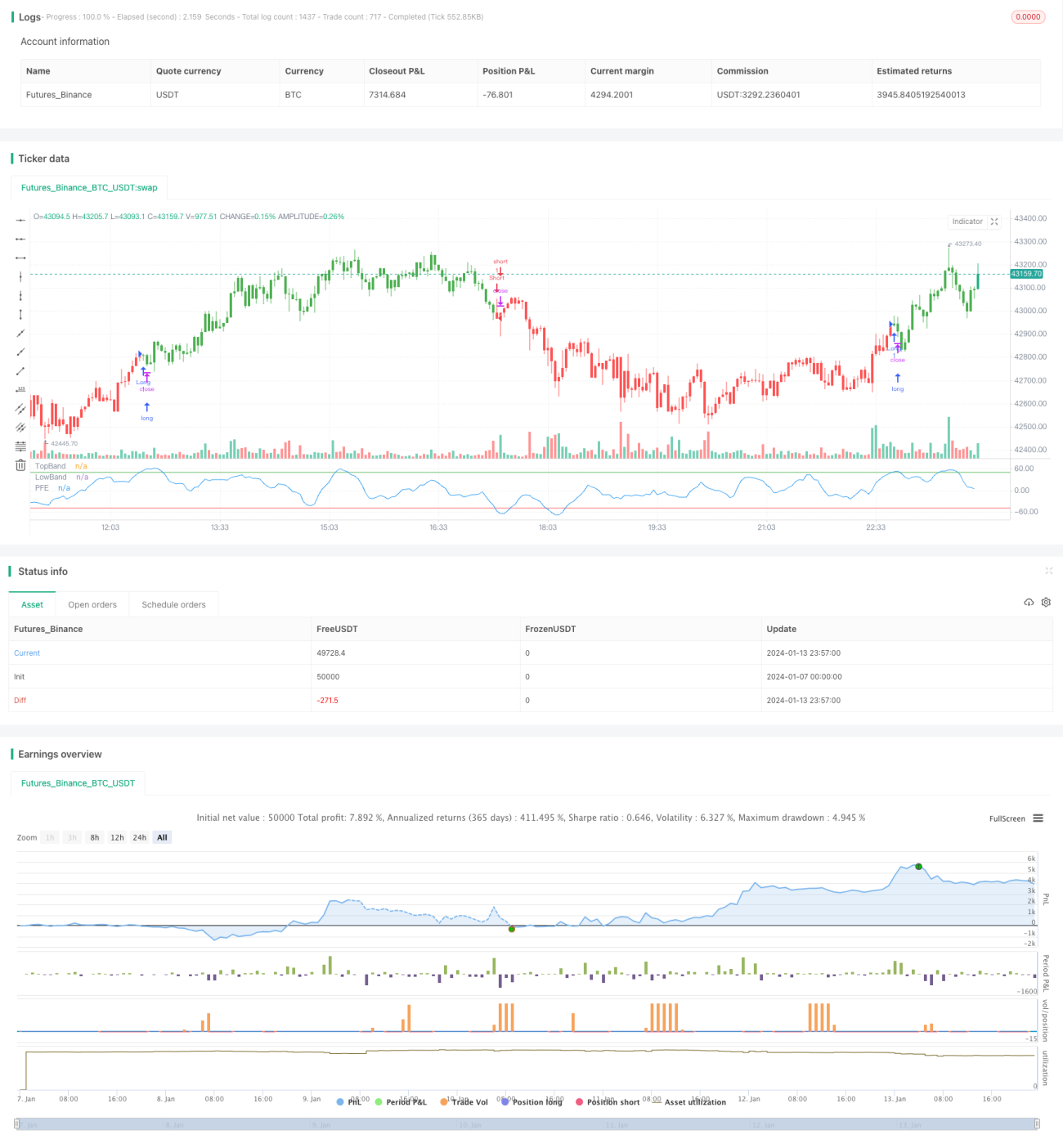
/*backtest
start: 2024-01-07 00:00:00
end: 2024-01-14 00:00:00
period: 3m
basePeriod: 1m
exchanges: [{"eid":"Futures_Binance","currency":"BTC_USDT"}]
*/

//@version=2
////////////////////////////////////////////////////////////
//  Copyright by HPotter v1.0 29/09/2017
// The Polarized Fractal Efficiency (PFE) indicator measures the efficiency - 1