
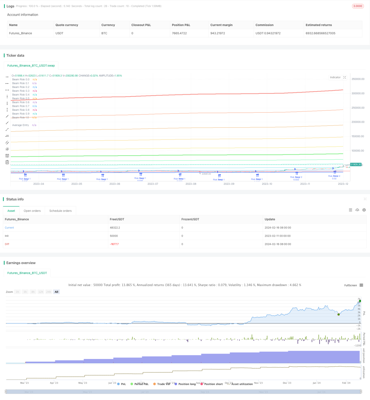
この戦略は,ベン・コウエンのリスクレベル理論に基づいており,BEAM波段のレベルを使用して同様の方法を実現することを目指しています.BEAM波段の上の境界は,対数をとった後の200週間の移動平均であり,下の境界は200週間の移動平均そのものです.これは,私たちに0から1の範囲を与えます.価格が0.5波段以下であるとき,買取命令が発せられます.価格が0.5波段以上であるとき,売り出せる命令が発せられます.
この戦略は主にベン・コウエンが提唱したBEAM波段理論に依存している.BTCの価格の変化に応じて,価格を0から1の間の10の領域に分けることができ,この10の領域は10の異なるリスクレベルを表している.レベル0は200週間の移動平均に近い価格を表し,リスクは最小である.レベル5は価格が中値領域にあることを表し,レベル10は上位に近い価格を表し,リスクは最大である.
価格が低値に下落すると,この戦略は徐々に買いポジションを拡大する.具体的には,価格が0から0.5の波段にある場合,戦略設定された毎月の特定の日に買い指示が発行され,購入金額は波段番号の減少に伴い徐々に増加する.例えば,波段5では,購入金額は月間DCA総額の20%であり,波段1では,購入金額は月間DCA総額の100%に増加する.
価格が上昇して高値に達すると,この戦略は徐々にポジションを小さくする.具体的には,価格が0.5波段を超えると,比例して売り命令が発行され,売りポジションは波段番号の増加に伴い徐々に大きくなる.例えば波段6時,6.67%を売り;波段10時,すべてのポジションを売り.
このBEAM波段DCAコスト平均策の最大の利点は,BTCの波動的な取引の特性を充分利用することであり,BTC価格が低谷に達するときに下下を押して,価格がピークに達するときに利益を得ることである.このやり方は,購入または販売の良い機会を逃さない.具体的利点は以下の通りです.
総括すると,これはBTCの波動的な状況で長期的に安定した利益を得ることができる精巧なパラメータ調節戦略である.
BEAM波段DCA戦略は多くの利点があるものの,注意すべき潜在的なリスクもあります.主なリスク点は以下の通りです.
リスクを下げるには,以下の措置を講じます.
この戦略は,上記のリスクポイントを考慮して,以下のような点で最適化できます.
戦略の安定性や安全性を大幅に向上させることができる.
BEAM波段DCAコスト平均戦略は,実戦に非常に価値のある量化戦略である.BEAM理論を利用して取引決定を導き,コスト平均モデルで購入コストを制御することに成功している.同時に,リスク管理にも注意し,損失拡大を防ぐために止損点を設定している.パラメータ最適化とモジュール増設により,この戦略は,BTC市場の長期の安定した収益を得るために,量化取引の重要なツールとなり得る.
/*backtest
start: 2023-02-11 00:00:00
end: 2024-02-17 00:00:00
period: 1d
basePeriod: 1h
exchanges: [{"eid":"Futures_Binance","currency":"BTC_USDT"}]
*/
// © gjfsdrtytru - BEAM DCA Strategy {
// Based on Ben Cowen's risk level strategy, this aims to copy that method but with BEAM band levels.
// Upper BEAM level is derived from ln(price/200W MA)/2.5, while the 200W MA is the floor price. This is our 0-1 range.
// Buy limit orders are set at the < 0.5 levels and sell orders are set at the > 0.5 level.
//@version=5
strategy(
title = "BEAM DCA Strategy Monthly",
shorttitle = "BEAM DCA M",
overlay = true,
pyramiding = 500,
default_qty_type = strategy.percent_of_equity,
default_qty_value = 0,
initial_capital = 0) //}
// Inputs { ————————————————————————————————————————————————————————————————————
T_ceiling = input.string("Off", "Diminishing Returns", ["Off","Linear","Parabolic"], "Account for diminishing returns as time increases")
day = input.int(1, "DCA Day of Month",1,28,1,"Select day of month for buy orders.")
DCAamount = input.int(1000,"DCA Amount",400,tooltip="Enter the maximum amount you'd be willing to DCA for any given month.")
T_buy = input(true,"Buy Orders","Toggle buy orders.")
T_sell = input(true,"Sell Orders","Toggle sell orders.")
// Time period
testStartYear = input.int(2018, title="Backtest Start Year", minval=2010,maxval=2100,group="Backtest Period")
testStartMonth = input.int(1, title="Backtest Start Month", minval=1, maxval=12, group="Backtest Period")
testStartDay = input.int(1, title="Backtest Start Day", minval=1, maxval=31, group="Backtest Period")
testPeriodLen = input.int(9999, title="Backtest Period (days)", minval=1, group="Backtest Period",tooltip="Days until strategy ends") * 86400000 // convert days into UNIX time
testPeriodStart = timestamp(testStartYear,testStartMonth,testStartDay,0,0)
testPeriodStop = testPeriodStart + testPeriodLen
testPeriod() => true
// ——————————————————————————————————————————————————————————————————————————— }
// Diminishing Returns { ———————————————————————————————————————————————————————
x = bar_index + 1
assetDivisor= 2.5
switch
T_ceiling == "Linear" => assetDivisor:= 3.50542 - 0.000277696 * x
T_ceiling == "Parabolic"=> assetDivisor:= -0.0000001058992338 * math.pow(x,2) + 0.000120729 * x + 3.1982
// ——————————————————————————————————————————————————————————————————————————— }
// Risk Levels { ———————————————————————————————————————————————————————————————
cycleLen = 1400
getMaLen() =>
if bar_index < cycleLen
bar_index + 1
else
cycleLen
// Define Risk Bands
price = close
riskLow = ta.sma(price,getMaLen())
risk1 = riskLow * math.exp((assetDivisor)*0.1)
risk2 = riskLow * math.exp((assetDivisor)*0.2)
risk3 = riskLow * math.exp((assetDivisor)*0.3)
risk4 = riskLow * math.exp((assetDivisor)*0.4)
risk5 = riskLow * math.exp((assetDivisor)*0.5)
risk6 = riskLow * math.exp((assetDivisor)*0.6)
risk7 = riskLow * math.exp((assetDivisor)*0.7)
risk8 = riskLow * math.exp((assetDivisor)*0.8)
risk9 = riskLow * math.exp((assetDivisor)*0.9)
riskHigh = riskLow * math.exp((assetDivisor))
// Plot Risk Bands
p_low = plot(riskLow, "Beam Risk 0.0",color.new(#0042F0,50),3,editable=false)
p_band1 = plot(risk1, "Beam Risk 0.1",color.new(#0090F5,20),1,editable=false)
p_band2 = plot(risk2, "Beam Risk 0.2",color.new(#00C6DB,20),1,editable=false)
p_band3 = plot(risk3, "Beam Risk 0.3",color.new(#00F5BD,20),1,editable=false)
p_band4 = plot(risk4, "Beam Risk 0.4",color.new(#00F069,20),1,editable=false)
p_band5 = plot(risk5, "Beam Risk 0.5",color.new(#00DB08,50),3,editable=false)
p_band6 = plot(risk6, "Beam Risk 0.6",color.new(#E8D20C,20),1,editable=false)
p_band7 = plot(risk7, "Beam Risk 0.7",color.new(#F2B40C,20),1,editable=false)
p_band8 = plot(risk8, "Beam Risk 0.8",color.new(#DC7A00,20),1,editable=false)
p_band9 = plot(risk9, "Beam Risk 0.9",color.new(#F2520C,20),1,editable=false)
p_band10 = plot(riskHigh, "Beam Risk 1.0",color.new(#F01102,50),3,editable=false)
// ——————————————————————————————————————————————————————————————————————————— }
// Order Execution { ———————————————————————————————————————————————————————————
band5 = price<risk5 and price>risk4
band4 = price<risk4 and price>risk3
band3 = price<risk3 and price>risk2
band2 = price<risk2 and price>risk1
band1 = price<risk1
// DCA buy order weights
y = DCAamount / 5
switch
band5 => y:= y * 1
band4 => y:= y * 2
band3 => y:= y * 3
band2 => y:= y * 4
band1 => y:= y * 5
// Contracts per order
contracts =(y/price)
if testPeriod()
// Buy orders
if T_buy == true
if dayofmonth == day
strategy.entry("Risk Band 5",strategy.long,qty=contracts,when=band5)
strategy.entry("Risk Band 4",strategy.long,qty=contracts,when=band4)
strategy.entry("Risk Band 3",strategy.long,qty=contracts,when=band3)
strategy.entry("Risk Band 2",strategy.long,qty=contracts,when=band2)
strategy.entry("Risk Band 1",strategy.long,qty=contracts,when=band1)
// Sell orders
if T_sell == true
if strategy.opentrades > 5
strategy.exit("Risk Band 6",qty_percent=6.67,limit=risk6)
strategy.exit("Risk Band 7",qty_percent=14.28,limit=risk7)
strategy.exit("Risk Band 8",qty_percent=25.00,limit=risk8)
strategy.exit("Risk Band 9",qty_percent=44.44,limit=risk9)
strategy.exit("Risk Band 10",qty_percent=100,limit=riskHigh)
// ——————————————————————————————————————————————————————————————————————————— }
// Info { ——————————————————————————————————————————————————————————————————————
// Line plot of avg. entry price
plot(strategy.position_size > 0 ? strategy.position_avg_price : na,"Average Entry",color.red,trackprice=true,editable=false)
// Unrealised PNL
uPNL = price/strategy.position_avg_price
// Realised PNL
realPNL = 0.
for i = 0 to strategy.closedtrades-1
realPNL += strategy.closedtrades.profit(i)
// Size of open position in ($)
openPosSize = 0.
for i = 0 to strategy.opentrades-1
openPosSize += strategy.opentrades.size(i) * strategy.position_avg_price
// Size of closed position in ($)
closePosSize = 0.
if strategy.closedtrades > 0
for i = 0 to strategy.closedtrades-1
closePosSize += strategy.closedtrades.size(i) * strategy.closedtrades.entry_price(i)
invested = openPosSize+closePosSize // Total capital ($) put into strategy
equity = openPosSize+closePosSize+strategy.openprofit+realPNL // Total current equity ($) in strategy (counting realised PNL)
ROI = (equity-invested) / invested * 100 // ROI of strategy (compare capital invested to excess return)
// // Info Table
// var table table1 = table.new(position.bottom_right,2,9,color.black,color.gray,1,color.gray,2)
// table.cell(table1,0,0,"Capital Invested", text_color=color.white,text_halign=text.align_right)
// table.cell(table1,0,1,"Open Position", text_color=color.white,text_halign=text.align_right)
// table.cell(table1,0,2,"Average Entry", text_color=color.white,text_halign=text.align_right)
// table.cell(table1,0,3,"Last Price", text_color=color.white,text_halign=text.align_right)
// table.cell(table1,0,4,"Open PNL (%)", text_color=color.white,text_halign=text.align_right)
// table.cell(table1,0,5,"Open PNL ($)", text_color=color.white,text_halign=text.align_right)
// table.cell(table1,0,6,"Realised PNL ($)", text_color=color.white,text_halign=text.align_right)
// table.cell(table1,0,7,"Total Equity", text_color=color.white,text_halign=text.align_right)
// table.cell(table1,0,8,"Strategy ROI", text_color=color.white,text_halign=text.align_right)
// table.cell(table1,1,0,"$" + str.tostring(invested, "#,###.00"), text_halign=text.align_right,text_color = color.white)
// table.cell(table1,1,1,"$" + str.tostring(openPosSize, "#,###.00"), text_halign=text.align_right,text_color = color.white)
// table.cell(table1,1,2,"$" + str.tostring(strategy.position_avg_price, "#,###.00"), text_halign=text.align_right,text_color = color.white)
// table.cell(table1,1,3,"$" + str.tostring(price, "#,###.00"), text_halign=text.align_right,text_color = color.white)
// table.cell(table1,1,4, str.tostring((uPNL-1)*100, "#,###.00") + "%",text_halign=text.align_right,text_color = uPNL > 1 ? color.lime : color.red)
// table.cell(table1,1,5,"$" + str.tostring(strategy.openprofit, "#,###.00"), text_halign=text.align_right,text_color = uPNL > 1 ? color.lime : color.red)
// table.cell(table1,1,6,"$" + str.tostring(realPNL, "#,###.00"), text_halign=text.align_right,text_color = color.white)
// table.cell(table1,1,7,"$" + str.tostring(equity, "#,###.00"), text_halign=text.align_right,text_color = color.white)
// table.cell(table1,1,8, str.tostring(ROI, "#,###.00") + "%",text_halign=text.align_right,text_color = ROI > 1 ? color.lime : color.red)
// // ——————————————————————————————————————————————————————————————————————————— }