시계열 분해 및 볼륨 가중치를 기반으로 한 볼린저 밴드 기술 지표 전략

1
Follow
1778
Followers
개요
이 전략은 시간 순서 분해, 거래량 가중 평균 가격, 브린 밴드 및 델타 (OBV-PVT) 4 가지 기술 지표를 결합하여 가격 동향, 과매매 과매매의 다차원 판단을 가능하게 한다.
전략 원칙
- 가격의 잡음과 주기성을 제거하는 시간 순서를 사용하여 더 정확한 추세를 판단합니다.
- 이 트렌드 라인을 바탕으로 거래량 가중된 새로운 가격을 계산합니다.
- 종결 가격의 브린 대역 비율 폭 BB%B 지표를 계산하여 과매매를 판단합니다.
- OBV-PVT의 변화량 델타 (Delta) 의 브린 대역의 퍼센티지 폭을 계산하여 측정값의 오차를 판단하는 기준으로;
- 수량 가격 지표의 다공간 교차와 브린 벨트 지표의 오버오프 회수로 거래 신호를 생성한다.
우위 분석
- 가격, 거래량, 통계적 특징에 대한 다양한 판단과 함께 전략적 강점을 갖추고 있습니다.
- BB%B와 델타 (OBV-PVT) 의 결합은 단기적인 과매매 현상을 더 잘 판단할 수 있다.
- 양과 가격의 교차 신호는 일부 노이즈 거래점을 필터링했다.
위험 분석
- 변수 설정이 너무 복잡해서 조정하기가 쉽지 않습니다.
- 단기 간격의 진동으로 인해 손실이 증가할 수 있습니다.
- 하지만, 이 경우, 이 값이 완전히 잘못된 신호를 필터링할 수 없습니다.
평균선 주기, 브린 대폭, 그리고 리스크/손실 비율을 조정하여 전략을 최적화하여 거래 빈도를 낮추는 동시에 단일 거래의 수익률을 높일 수 있다.
요약하다
이 전략은 종합적으로 타임 시퀀스 분해, 브린 밴드 지표, OBV 지표 등의 여러 가지 분석 도구를 사용하여 수량 관계, 통계적 특성 및 추세 판단의 유기적 결합을 통해 단기 여진을 식별하여 시장의 주요 추세를 효과적으로 잡을 수 있습니다. 또한 특정 위험이 있으며, 파라미터를 통해 최적의 상태에 도달하기 위해 조정해야합니다.
Source
Pine
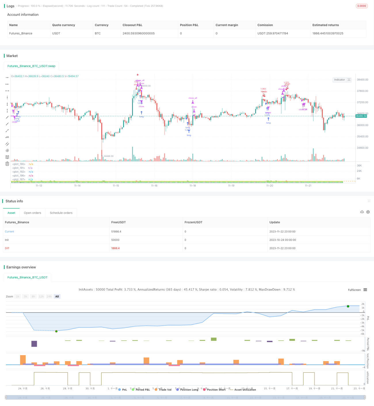
/*backtest
start: 2023-10-24 00:00:00
end: 2023-11-23 00:00:00
period: 1h
basePeriod: 15m
exchanges: [{"eid":"Futures_Binance","currency":"BTC_USDT"}]
*/

// This source code is subject to the terms of the Mozilla Public License 2.0 at https://mozilla.org/MPL/2.0/
//// This source code is subject to the terms of the Mozilla Public License 2.0 at https://mozilla.org/MPL/2.0/
// © oakwhiz and tathal
Strategy parameters
Related strategies
Comment
All comments (0)
No data
- 1