BEAM 밴드를 기반으로 한 BTC달러 비용 평균화 전략

개요
이 전략은 벤 코웬의 위험 레벨 이론에 기반을 두고 있으며, BEAM 파장의 레벨을 사용하여 유사한 방법을 구현하는 것을 목표로 한다. BEAM 파장의 상한은 대칭을 따온 200주 이동 평균이고, 하한은 200주 이동 평균이다. 이것은 우리에게 0에서 1의 범위를 준다. 가격이 0.5 파장의 아래에 있을 때, 구매 지시가 발령되고, 가격이 0.5 파장의 위에 있을 때, 판매 지시가 발령된다.
전략 원칙
이 전략은 주로 벤 코웬 (Ben Cowen) 이 제시한 BEAM 파동 이론에 의존한다. BTC의 가격 변화에 따라 가격을 0에서 1 사이의 10개의 영역으로 나눌 수 있으며, 이 10개의 영역은 10개의 다른 위험 레벨을 나타낸다. 0 레벨은 200주 이동 평균에 가까운 가격을 나타내고, 위험은 최소이다.
가격이 하락할 때, 이 전략은 점진적으로 구매 포지션을 증가시킨다. 구체적으로, 가격이 0에서 0.5의 파동에 있다면, 전략 설정된 매월의 특정 날에 구매 지시가 발령되며, 구매 금액은 파동 번호가 줄어들면서 점진적으로 증가한다. 예를 들어, 파동 5시에는 구매 금액이 월 DCA 총액의 20%이며, 파동 1시에는 구매 금액이 월 DCA 총액의 100%로 증가한다.
가격이 높은 지점으로 올라갈 때, 이 전략은 점진적으로 포지션을 줄인다. 구체적으로, 가격이 0.5 파도를 넘으면, 비율로 판매 지시가 발령되며, 판매 포지션은 파도 번호가 증가함에 따라 점진적으로 증가한다. 예를 들어, 파도 6 때, 6.67%를 판매; 파도 10 때, 모든 포지션을 판매한다.
우위 분석
이 BEAM 파동 DCA 비용 평균 전략의 가장 큰 장점은 BTC의 파동 거래의 특성을 최대한 활용하고 BTC 가격이 하락할 때 상쇄하고 가격이 상승할 때 수익을 창출한다는 것입니다. 이 방법은 구매하거나 판매 할 수있는 기회를 놓치지 않습니다. 구체적인 장점은 다음과 같습니다.
- BEAM 이론을 이용해서 자산의 과소평가 정도를 판단하고, 과학적인 위험을 회피하는 방법
- BTC의 변동성을 최대한 활용하여 가장 정확한 구매와 판매 기회를 잡을 수 있습니다.
- 비용평균을 적용하여 투자비용을 효율적으로 통제하고 장기적으로 안정적인 수익을 얻습니다.
- 자동으로 거래하고, 인적 개입이 필요없고, 운영의 위험을 줄여줍니다.
- 사용자 정의 가능한 매개 변수, 시장 변화에 적응할 수 있는 유연한 조정 전략.
종합적으로, 이것은 BTC의 불안정한 상황에서 장기적으로 안정적인 수익을 얻을 수 있는 정교한 변수 조절 전략입니다.
위험 분석
BEAM 대역 DCA 전략은 여러 장점이 있지만, 몇 가지 잠재적인 위험도 있습니다. 주요 위험점은 다음과 같이 요약할 수 있습니다.
- BEAM 이론과 파라미터 설정은 주관적인 판단에 의존하고 있으며, 잘못된 판단이 발생할 가능성이 있습니다.
- BTC의 추세는 예측하기 어렵고, 손실과 손실의 위험이 있습니다.
- 자동 거래는 시스템 장애와 파라미터 해킹에 취약합니다.
- 과도한 변동은 손실을 확대할 수 있습니다.
위험을 줄이기 위해 다음과 같은 조치를 취할 수 있습니다.
- BEAM 이론의 판단 정확성을 높이기 위해 최적화 파라미터 설정;
- 적당히 포지션 규모를 축소하여 단편적 손실을 줄여주기
- 자동화 거래의 위험성을 줄이기 위해 과잉과 오류 용도를 높여줍니다.
- 단독 손실이 너무 커지는 것을 방지하기 위해 스톱포인트를 설정하십시오.
최적화 방향
위와 같은 위험 요소를 고려하여, 이 전략은 다음과 같은 측면에서 최적화될 수 있습니다.
- BEAM 이론의 매개 변수를 최적화: 로그법 매개 변수, 재측정 주기 등을 조정하여 모델 판단의 정확도를 향상시킨다.
- 포지션 통제를 최적화: 월간 DCA 총액, 매매 비율 등을 조정하여 일회성 손실 위험을 제어합니다.
- 자동 거래 보안 모듈을 추가: 과잉 서버, 로컬 처리 등으로 설정하고, 오류 수용력을 향상시킵니다.
- 추가된 스톱로스 모듈: 역사적인 변동에 따라 합리적인 스톱로스를 설정하여 손실을 효과적으로 제어한다.
이러한 수단으로 전략의 안정성과 안전성을 크게 향상시킬 수 있습니다.
요약하다
BEAM 파동 DCA 비용 평균 전략은 매우 실전 가치가있는 양적 전략이다. BEAM 이론을 사용하여 거래 결정을 안내하는 데 성공하고, 비용 평균 모델에 의해 구매 비용을 제어한다. 동시에, 위험 관리에 주의를 기울이며, 손실을 방지하기 위해 스톱 스포트를 설정한다. 변수 최적화 및 모듈 추가로, 이 전략은 양적 거래의 중요한 도구가 될 수 있으며, BTC 시장의 장기적인 안정적인 수익을 얻을 수 있다.
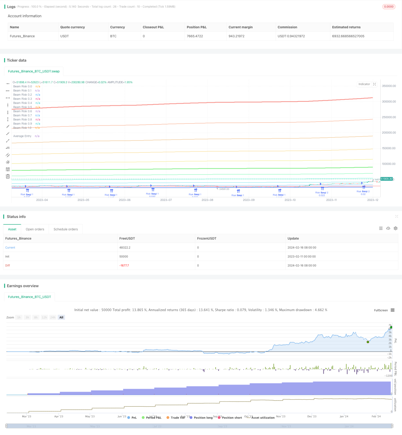
/*backtest
start: 2023-02-11 00:00:00
end: 2024-02-17 00:00:00
period: 1d
basePeriod: 1h
exchanges: [{"eid":"Futures_Binance","currency":"BTC_USDT"}]
*/

// © gjfsdrtytru - BEAM DCA Strategy {
// Based on Ben Cowen's risk level strategy, this aims to copy that method but with BEAM band levels.
// Upper BEAM level is derived from ln(price/200W MA)/2.5, while the 200W MA is the floor price. This is our 0-1 range.
// Buy limit orders are set at the < 0.5 levels and sell orders are set at the > 0.5 level.- 1