Chiến lược chỉ báo kỹ thuật Bollinger Bands dựa trên phân tích chuỗi thời gian và trọng số khối lượng


Ngày tạo: 2023-11-24 11:29:40 sửa đổi lần cuối: 2023-11-24 11:29:40
sao chép: 0 Số nhấp chuột: 698
1
tập trung vào
1617
Người theo dõi

Chiến lược chỉ báo kỹ thuật Bollinger Bands dựa trên phân tích chuỗi thời gian và trọng số khối lượng

Tổng quan

Chiến lược này kết hợp 4 chỉ số kỹ thuật phân tích theo trình tự thời gian, giá trung bình cân bằng khối lượng giao dịch, băng tần Brin và delta (OBV-PVT) để đưa ra phán đoán đa chiều về xu hướng giá, mua quá mức và bán quá mức.

Nguyên tắc chiến lược

  1. Sử dụng phân tích theo trình tự thời gian để loại bỏ tiếng ồn và chu kỳ trong giá, để có được xu hướng chính xác hơn;
  2. Dựa trên đường xu hướng này, tính giá mới có trọng lượng giao dịch;
  3. Tính toán tỷ lệ phần trăm chiều rộng của Brin với giá đóng cửa theo chỉ số BB% B để đánh giá quá mua quá bán;
  4. Tính phần trăm chiều rộng của dải Brinh của biến số Delta của OBV-PVT (OBV-PVT) như một tiêu chuẩn để xác định sai lệch giá trị;
  5. Tín hiệu giao dịch được tạo ra dựa trên sự giao thoa đa không gian của chỉ số giá trị và sự vượt qua và rút lui của chỉ số Brin.

Phân tích lợi thế

  1. Một chiến lược mạnh mẽ kết hợp với nhiều phán đoán về giá cả, khối lượng giao dịch và các đặc điểm thống kê;
  2. Kết hợp BB%B và Delta (OBV-PVT) sẽ giúp đánh giá tốt hơn về tình trạng quá mua và quá bán trong ngắn hạn.
  3. Một số điểm giao dịch đã bị lọc bởi tín hiệu giao dịch giá cả.

Phân tích rủi ro

  1. Thiết lập tham số quá phức tạp và không dễ điều chỉnh;
  2. Các trận động đất có thể làm tăng thiệt hại trong thời gian ngắn.
  3. Giá cả lệch không hoàn toàn lọc các tín hiệu sai lệch.

Các chiến lược có thể được tối ưu hóa bằng cách điều chỉnh chu kỳ đường trung bình, độ rộng của Brin và tỷ lệ lợi nhuận rủi ro để giảm tần suất giao dịch và tăng tỷ lệ lợi nhuận của một giao dịch.

Tóm tắt

Chiến lược tổng hợp sử dụng nhiều công cụ phân tích như phân giải chuỗi thời gian, chỉ số Brin, chỉ số OBV, thông qua sự kết hợp hữu cơ của quan hệ giá trị, tính thống kê và phán đoán xu hướng, để nhận diện các hậu quả ngắn hạn, có thể nắm bắt được xu hướng chính của thị trường. Tuy nhiên, cũng có một số rủi ro, cần điều chỉnh thông qua tham số để đạt được trạng thái tối ưu.
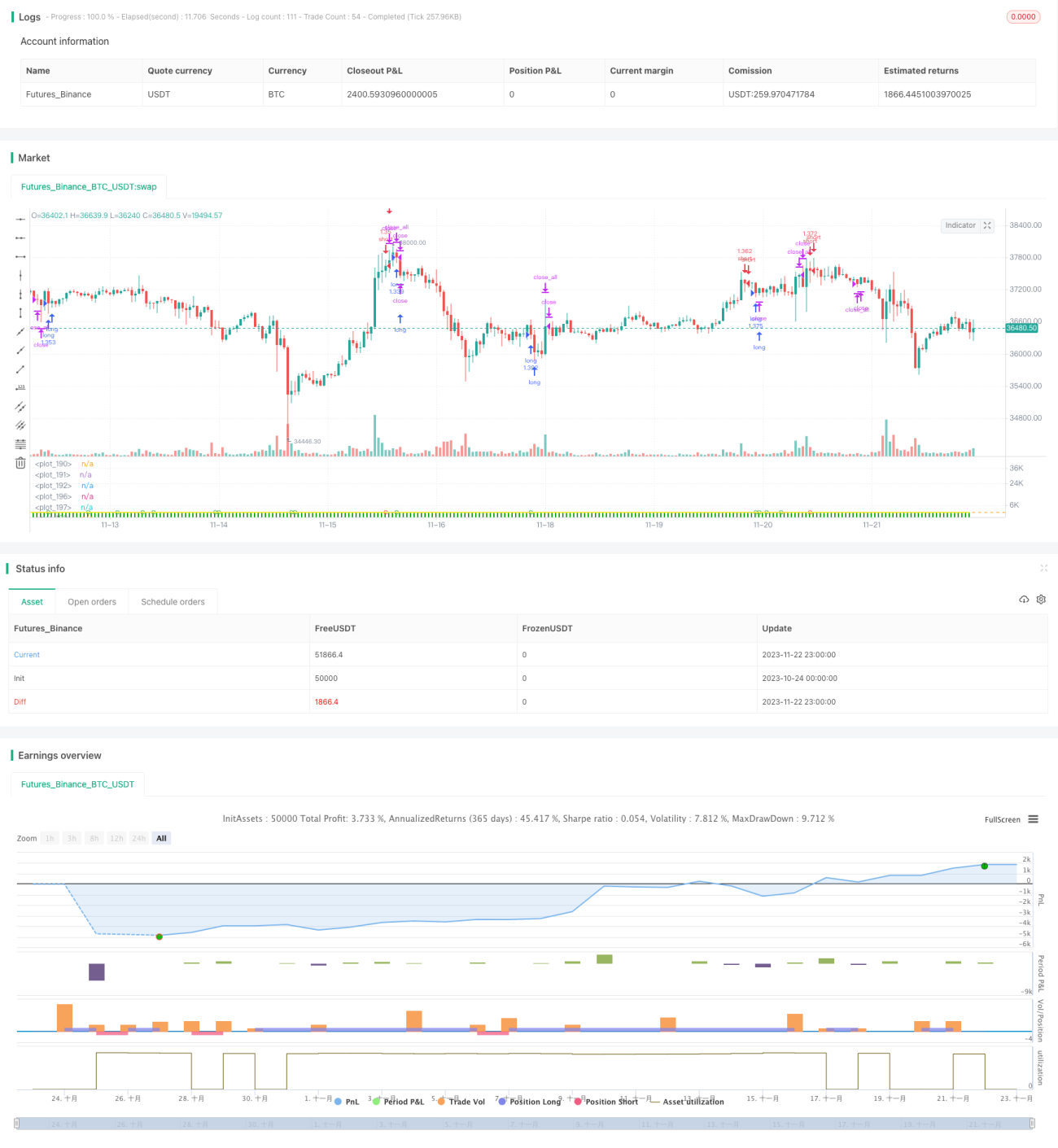
Mã nguồn chiến lược
/*backtest
start: 2023-10-24 00:00:00
end: 2023-11-23 00:00:00
period: 1h
basePeriod: 15m
exchanges: [{"eid":"Futures_Binance","currency":"BTC_USDT"}]
*/

// This source code is subject to the terms of the Mozilla Public License 2.0 at https://mozilla.org/MPL/2.0/
//// This source code is subject to the terms of the Mozilla Public License 2.0 at https://mozilla.org/MPL/2.0/
// © oakwhiz and tathal

//@version=4
strategy("BBPBΔ(OBV-PVT)BB", default_qty_type=strategy.percent_of_equity, default_qty_value=100)

startDate = input(title="Start Date", type=input.integer,
     defval=1, minval=1, maxval=31)
startMonth = input(title="Start Month", type=input.integer,
     defval=1, minval=1, maxval=12)
startYear = input(title="Start Year", type=input.integer,
     defval=2010, minval=1800, maxval=2100)

endDate = input(title="End Date", type=input.integer,
     defval=31, minval=1, maxval=31)
endMonth = input(title="End Month", type=input.integer,
     defval=12, minval=1, maxval=12)
endYear = input(title="End Year", type=input.integer,
     defval=2021, minval=1800, maxval=2100)

// Normalize Function
normalize(_src, _min, _max) =>
    // Normalizes series with unknown min/max using historical min/max.
    // _src      : series to rescale.
    // _min, _min: min/max values of rescaled series.
    var _historicMin =  10e10
    var _historicMax = -10e10
    _historicMin := min(nz(_src, _historicMin), _historicMin)
    _historicMax := max(nz(_src, _historicMax), _historicMax)
    _min + (_max - _min) * (_src - _historicMin) / max(_historicMax - _historicMin, 10e-10)
    

// STEP 2:
// Look if the close time of the current bar
// falls inside the date range
inDateRange = true
     
     
// Stop loss & Take Profit Section     
sl_inp = input(2.0, title='Stop Loss %')/100
tp_inp = input(4.0, title='Take Profit %')/100
 
stop_level = strategy.position_avg_price * (1 - sl_inp)
take_level = strategy.position_avg_price * (1 + tp_inp)

icreturn = false
innercandle = if (high < high[1]) and (low > low[1])
    icreturn := true

src = close

float change_src = change(src)
float i_obv = cum(change_src > 0 ? volume : change_src < 0 ? -volume : 0*volume)
float i_pvt = pvt

float result = change(i_obv - i_pvt)

float nresult = ema(normalize(result, -1, 1), 20)


length = input(20, minval=1)
mult = input(2.0, minval=0.001, maxval=50, title="StdDev")
basis = ema(nresult, length)
dev = mult * stdev(nresult, length)
upper = basis + dev
lower = basis - dev
bbr = (nresult - lower)/(upper - lower)


////////////////INPUTS///////////////////
lambda = input(defval = 1000, type = input.float, title = "Smoothing Factor (Lambda)", minval = 1)
leng = input(defval = 100, type = input.integer, title = "Filter Length", minval = 1)
srcc = close

///////////Construct Arrays///////////////
a = array.new_float(leng, 0.0) 
b = array.new_float(leng, 0.0)
c = array.new_float(leng, 0.0)
d = array.new_float(leng, 0.0)
e = array.new_float(leng, 0.0)
f = array.new_float(leng, 0.0)

/////////Initialize the Values///////////
//for more details visit:
//          https://asmquantmacro.com/2015/06/25/hodrick-prescott-filter-in-excel/

ll1 = leng-1
ll2 = leng-2

for i = 0 to ll1
    array.set(a,i, lambda*(-4))
    array.set(b,i, src[i])
    array.set(c,i, lambda*(-4))
    array.set(d,i, lambda*6 + 1)
    array.set(e,i, lambda)
    array.set(f,i, lambda)

array.set(d, 0,  lambda + 1.0)
array.set(d, ll1, lambda + 1.0)
array.set(d, 1,  lambda * 5.0 + 1.0)
array.set(d, ll2, lambda * 5.0 + 1.0)

array.set(c, 0 , lambda * (-2.0))
array.set(c, ll2, lambda * (-2.0))

array.set(a, 0 , lambda * (-2.0))
array.set(a, ll2, lambda * (-2.0))

//////////////Solve the optimization issue/////////////////////
float r = array.get(a, 0)
float s = array.get(a, 1)
float t = array.get(e, 0)
float xmult = 0.0

for i = 1 to ll2
    xmult := r / array.get(d, i-1) 
    array.set(d, i, array.get(d, i) - xmult * array.get(c, i-1))
    array.set(c, i, array.get(c, i) - xmult * array.get(f, i-1))
    array.set(b, i, array.get(b, i) - xmult * array.get(b, i-1))

    xmult := t / array.get(d, i-1)
    r     := s - xmult*array.get(c, i-1)
    array.set(d, i+1, array.get(d, i+1) - xmult * array.get(f, i-1))
    array.set(b, i+1, array.get(b, i+1) - xmult * array.get(b, i-1))
    
    s     := array.get(a, i+1)
    t     := array.get(e, i)

xmult := r / array.get(d, ll2)
array.set(d, ll1, array.get(d, ll1) - xmult * array.get(c, ll2))

x = array.new_float(leng, 0) 
array.set(x, ll1, (array.get(b, ll1) - xmult * array.get(b, ll2)) / array.get(d, ll1))
array.set(x, ll2, (array.get(b, ll2) - array.get(c, ll2) * array.get(x, ll1)) / array.get(d, ll2))

for j = 0 to leng-3
    i = leng-3 - j
    array.set(x, i, (array.get(b,i) - array.get(f,i)*array.get(x,i+2) - array.get(c,i)*array.get(x,i+1)) / array.get(d, i))


//////////////Construct the output///////////////////
o5 = array.get(x,0)

////////////////////Plottingd///////////////////////


TimeFrame = input('1', type=input.resolution)
start = security(syminfo.tickerid, TimeFrame, time)

//------------------------------------------------
newSession = iff(change(start), 1, 0)
//------------------------------------------------
vwapsum = 0.0
vwapsum := iff(newSession, o5*volume, vwapsum[1]+o5*volume)
volumesum = 0.0
volumesum := iff(newSession, volume, volumesum[1]+volume)
v2sum = 0.0
v2sum := iff(newSession, volume*o5*o5, v2sum[1]+volume*o5*o5)
myvwap = vwapsum/volumesum
dev2 = sqrt(max(v2sum/volumesum - myvwap*myvwap, 0))
Coloring=close>myvwap?color.green:color.red
av=myvwap
showBcol = input(false, type=input.bool, title="Show barcolors")
showPrevVWAP = input(false, type=input.bool, title="Show previous VWAP close")
prevwap = 0.0
prevwap := iff(newSession, myvwap[1], prevwap[1])
nprevwap= normalize(prevwap, 0, 1)

l1= input(20, minval=1)
src2 = close
mult1 = input(2.0, minval=0.001, maxval=50, title="StdDev")
basis1 = sma(src2, l1)
dev1 = mult1 * stdev(src2, l1)
upper1 = basis1 + dev1
lower1 = basis1 - dev1
bbr1 = (src - lower1)/(upper1 - lower1)

az = plot(bbr, "Δ(OBV-PVT)", color.rgb(0,153,0,0), style=plot.style_columns)
bz = plot(bbr1, "BB%B", color.rgb(0,125,125,50), style=plot.style_columns)
fill(az, bz, color=color.white)


deltabbr = bbr1 - bbr
oneline = hline(1)
twoline = hline(1.2)
zline = hline(0)
xx = input(.3)
yy = input(.7)
zz = input(-1)
xxx = hline(xx)
yyy = hline(yy)
zzz = hline(zz)
fill(oneline, twoline, color=color.red, title="Sell Zone")
fill(yyy, oneline, color=color.orange, title="Slightly Overbought")
fill(yyy, zline, color=color.white, title="DO NOTHING ZONE")
fill(zzz, zline, color=color.green, title="GO LONG ZONE")

l20 = crossover(deltabbr, 0)
l30 = crossunder(deltabbr, 0)
l40 = crossover(o5, 0)
l50 = crossunder(o5, 0)


z1 = bbr1 >= 1
z2 = bbr1 < 1 and bbr1 >= .7
z3 = bbr1 < .7 and bbr1 >= .3
z4 = bbr1 < .3 and bbr1 >= 0
z5 = bbr1 < 0
a1 = bbr >= 1
a2 = bbr < 1 and bbr >= .7

a4 = bbr < .3 and bbr >= 0
a5 = bbr < 0
b4 = deltabbr < .3 and deltabbr >= 0
b5 = deltabbr < 0
c4 = o5 < .3 and o5 >= 0
c5 = o5 < 0
b1 = deltabbr >= 1
b2 = deltabbr < 1 and o5 >= .7
c1 = o5 >= 1
c2 = o5 < 1 and o5 >= .7

///

n = input(16,"Period")
H = highest(hl2,n)
L = lowest(hl2,n)
hi = H[1]
lo = L[1]
up = high>hi
dn = low<lo
lowerbbh = lowest(10)[1]
bbh = (low == open ?  open < lowerbbh ? open < close ? close > ((high[1] - low[1]) / 2) + low[1] :na  : na : na)


plot(normalize(av,-1,1), linewidth=2, title="Trendline", color=color.yellow)


long5 = close < av and av[0] > av[1]
sell5 = close > av

cancel = false
if open >= high[1]
    cancel = true


long = (long5 or z5 or a5) and (icreturn or bbh or up)
sell = ((z1 or a1) or (l40 and l20)) and (icreturn or dn) and (c1 or b1)
short = ((z1 or z2 or a1 or sell5) and (l40 or l20)) and icreturn
buy= (z5 or z4 or a5 or long5) and (icreturn or dn)


plotshape(long and not sell ? -0.5 : na, title="Long", location=location.absolute, style=shape.circle, size=size.tiny, color=color.green, transp=0)
plotshape(short and not sell? 1 : na, title="Short", location=location.absolute, style=shape.circle, size=size.tiny, color=color.red, transp=0)


if (inDateRange)
    strategy.entry("long", true, when = long )

if (inDateRange) and (strategy.position_size > 0)
    strategy.close_all(when = sell or cancel)
    

if (inDateRange)
    strategy.entry("short", false, when = short )

if (inDateRange) and (strategy.position_size < 0)
    strategy.close_all(when = buy)