Tài nguyên đang được tải lên... tải...

Chiến lược giao dịch Bollinger Percentage Bands

Tác giả:ChaoZhang, Ngày: 2023-12-11 11:14:53
Tags:

Tổng quan

Chiến lược này dựa trên chỉ số Bollinger Bands, kết hợp với đường trung bình động và chỉ số kỹ thuật ATR, để thực hiện một hệ thống đột phá ngắn hạn. Chiến lược tính toán vị trí tỷ lệ phần trăm tương đối của giá trong kênh Bollinger Bands để đánh giá các tình huống mua quá mức và bán quá mức, kết hợp với các mức cao và thấp mới để tạo ra các tín hiệu giao dịch.

Chiến lược logic

Tính toán kênh Bollinger Bands và tỷ lệ phần trăm tương đối của giá trong kênh
Tính toán trung bình động riêng biệt cho giá mở, đóng, cao và thấp
Tính toán chỉ số ATR và thiết lập các đường dừng lỗ kết hợp với ATR
Xác định xem giá có gần mức cao mới hay mức thấp mới
Kết hợp mức cao và thấp hàng năm để đánh giá xu hướng khung thời gian lớn hơn
Tạo tín hiệu giao dịch dựa trên thay đổi tỷ lệ phần trăm Bollinger Bands và mức cao/mức thấp mới

Chiến lược này sử dụng kênh Bollinger Bands để đánh giá sự biến động của thị trường, với chiều rộng kênh được xác định bởi độ lệch chuẩn. Các tín hiệu mua được tạo ra khi giá phá vỡ dưới dải dưới, và bán tín hiệu khi giá phá vỡ trên dải trên. Mức trung bình chuyển động có thể làm mịn biến động Bollinger và giảm phá vỡ sai. Chỉ số ATR kết hợp với stop loss để cố định quy mô stop loss. Mức cao/mức thấp mới giúp tránh đuổi theo đỉnh và giới hạn giảm. Mức cao/mức thấp hàng năm lọc ra sự củng cố khung thời gian lớn hơn.

Ưu điểm

Bộ lọc Bollinger Bands nghiêm ngặt giúp giảm tín hiệu sai
Mức trung bình động làm mượt giá và xác định xu hướng thực sự
Chỉ số ATR theo dõi động stop loss và giới hạn lỗ giao dịch đơn
Mức cao/mức thấp mới và mức cao/mức thấp hàng năm làm cho tín hiệu đáng tin cậy hơn
Sự kết hợp hiệu quả của nhiều chỉ số cải thiện hiệu quả

Rủi ro và giải pháp

Các thông số Bollinger Bands không chính xác có thể gây ra sự phá vỡ sai quá mức, nên thử nghiệm các kết hợp thông số khác nhau để có kết quả tốt nhất
Giá tham chiếu đóng cửa có thể dẫn đến rút vốn vượt quá phạm vi dừng lỗ được thiết lập ATR, xem xét sử dụng giá cao / thấp biến động hơn để tính phần trăm
Bộ lọc Bollinger nghiêm ngặt có thể bỏ lỡ một số cơ hội xu hướng dài hạn, thư giãn bộ lọc và thời gian giữ phù hợp
Chỉ số ATR theo dõi biến động giá lớn chậm, xem xét các biện pháp biến động tần số cao hơn như phạm vi thực sự
Sự đột phá cao/ thấp mới dễ bị xáo trộn bởi tiếng ồn ngắn hạn, đánh giá ý nghĩa thống kê và tính bền vững của xu hướng

Hướng dẫn tối ưu hóa

Kiểm tra các kết hợp tham số khác nhau để xác định các tham số Bollinger tối ưu và chiều dài trung bình động
Sử dụng kết hợp mô hình kết hợp các tham số Bollinger hoặc đường trung bình động khác nhau
Kiểm tra độ bền trên các khung thời gian và sản phẩm khác nhau, cải thiện khả năng thích nghi
Kết hợp nhiều tín hiệu khung thời gian cao hơn như tín hiệu Bollinger hàng ngày hoặc các yếu tố theo mùa
Đánh giá các cơ hội theo xu hướng để mở rộng phạm vi chiến lược và lợi nhuận

Kết luận

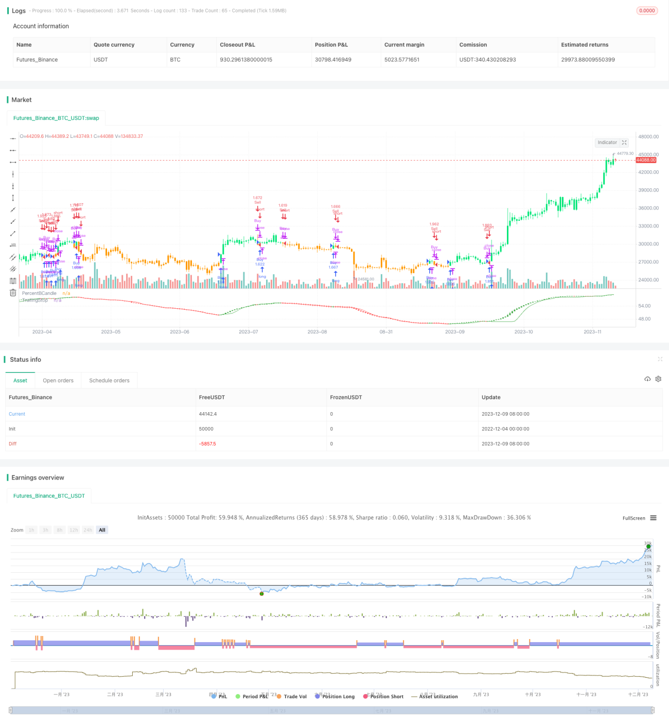
Chiến lược này kết hợp hiệu quả các dải tỷ lệ phần trăm Bollinger, đường trung bình động, chỉ số ATR, mức cao / thấp mới và mức cao / thấp hàng năm để xây dựng một hệ thống giao dịch breakout ngắn hạn tương đối nghiêm ngặt và hiệu quả. Ưu điểm nổi bật của nó nằm trong việc sử dụng các công cụ khác nhau để giảm tiếng ồn và xác định các tín hiệu xu hướng thực sự. Tất nhiên chiến lược cũng phải đối mặt với một số khó khăn điều chỉnh tham số và cơ hội bị bỏ lỡ trong điều kiện nghiêm ngặt.

/*backtest
start: 2022-12-04 00:00:00
end: 2023-12-10 00:00:00
period: 1d
basePeriod: 1h
exchanges: [{"eid":"Futures_Binance","currency":"BTC_USDT"}]
*/

// This source code is subject to the terms of the Mozilla Public License 2.0 at https://mozilla.org/MPL/2.0/
// © HeWhoMustNotBeNamed

//@version=4
strategy("Bollinger %B Candles Strategy", overlay=false, initial_capital = 1000, default_qty_type = strategy.percent_of_equity, default_qty_value = 100, commission_type = strategy.commission.percent, pyramiding = 1, commission_value = 0.01, calc_on_order_fills = true)

BBLength = input(100, minval=1, step=1)
StdDev = 10
useMovingAverage = input(true)
MAType = input(title="Moving Average Type", defval="rma", options=["ema", "sma", "hma", "rma", "vwma", "wma"])
lookbackPeriod = input(22, minval=10, step=10)
colorByPreviousClose = input(true)

AtrMAType = input(title="Moving Average Type", defval="hma", options=["ema", "sma", "hma", "rma", "vwma", "wma"])
AtrLength = input(10)
AtrMult = input(4)
wicks = input(false)

considerYearlyHighLow = input(false)
considerNewLongTermHighLows = input(false)
shortHighLowPeriod = 100
longHighLowPeriod = 200
tradeDirection = input(title="Trade Direction", defval=strategy.direction.all, options=[strategy.direction.all, strategy.direction.long, strategy.direction.short])

backtestYears = input(10, minval=1, step=1)


//////////////////////////////////// Calculate new high low condition //////////////////////////////////////////////////
f_calculateNewHighLows(shortHighLowPeriod, longHighLowPeriod, considerNewLongTermHighLows)=>
    newHigh = highest(shortHighLowPeriod) == highest(longHighLowPeriod) or not considerNewLongTermHighLows
    newLow = lowest(shortHighLowPeriod) == lowest(longHighLowPeriod) or not considerNewLongTermHighLows
    [newHigh,newLow]

//////////////////////////////////// Calculate Yearly High Low //////////////////////////////////////////////////
f_getYearlyHighLowCondition(considerYearlyHighLow)=>
    yhigh = security(syminfo.tickerid, '12M', high[1]) 
    ylow = security(syminfo.tickerid, '12M', low[1]) 
    yhighlast = yhigh[365]
    ylowlast = ylow[365]
    yhighllast = yhigh[2 * 365]
    ylowllast = ylow[2 * 365]
    
    yearlyTrendUp = na(yhigh)? true : na(yhighlast)? close > yhigh : na(yhighllast)? close > max(yhigh,yhighlast) : close > max(yhigh, min(yhighlast, yhighllast))
    yearlyHighCondition = (  (na(yhigh) or na(yhighlast) ? true : (yhigh > yhighlast) ) and ( na(yhigh) or na(yhighllast) ? true : (yhigh > yhighllast))) or yearlyTrendUp or not considerYearlyHighLow
    yearlyTrendDown = na(ylow)? true : na(ylowlast)? close < ylow : na(ylowllast)? close < min(ylow,ylowlast) : close < min(ylow, max(ylowlast, ylowllast))
    yearlyLowCondition = (  (na(ylow) or na(ylowlast) ? true : (ylow < ylowlast) ) and ( na(ylow) or na(ylowllast) ? true : (ylow < ylowllast))) or yearlyTrendDown or not considerYearlyHighLow
    
    label_x = time+(60*60*24*1000*1)
    [yearlyHighCondition,yearlyLowCondition]

f_getMovingAverage(source, MAType, length)=>
    ma = sma(source, length)
    if(MAType == "ema")
        ma := ema(source,length)
    if(MAType == "hma")
        ma := hma(source,length)
    if(MAType == "rma")
        ma := rma(source,length)
    if(MAType == "vwma")
        ma := vwma(source,length)
    if(MAType == "wma")
        ma := wma(source,length)
    ma

inDateRange = true
[yearlyHighCondition,yearlyLowCondition] = f_getYearlyHighLowCondition(considerYearlyHighLow)
[newHighS,newLowS] = f_calculateNewHighLows(shortHighLowPeriod, longHighLowPeriod, considerNewLongTermHighLows)
[middleclose, upperclose, lowerclose] = bb(close, BBLength, StdDev)
[middleopen, upperopen, loweropen] = bb(open, BBLength, StdDev)
[middlehigh, upperhigh, lowerhigh] = bb(high, BBLength, StdDev)
[middlelow, upperlow, lowerlow] = bb(low, BBLength, StdDev)

percentBClose = (close - lowerclose)*100/(upperclose-lowerclose)
percentBOpen = (open - loweropen)*100/(upperopen-loweropen)
percentBHigh = (high - lowerhigh)*100/(upperhigh-lowerhigh)
percentBLow = (low - lowerlow)*100/(upperlow-lowerlow)

percentBMAClose = f_getMovingAverage(percentBClose, MAType, lookbackPeriod)
percentBMAOpen = f_getMovingAverage(percentBOpen, MAType, lookbackPeriod)
percentBMAHigh = f_getMovingAverage(percentBHigh, MAType, lookbackPeriod)
percentBMALow = f_getMovingAverage(percentBLow, MAType, lookbackPeriod)

newOpen = useMovingAverage? percentBMAOpen : percentBOpen
newClose = useMovingAverage? percentBMAClose : percentBClose
newHigh = useMovingAverage? percentBMAHigh : percentBHigh
newLow = useMovingAverage? percentBMALow : percentBLow

truerange = max(newHigh, newClose[1]) - min(newLow, newClose[1])

averagetruerange = f_getMovingAverage(truerange, AtrMAType, AtrLength)
atr = averagetruerange * AtrMult

longStop = newClose - atr
longStopPrev = nz(longStop[1], longStop)
longStop := (wicks ? newLow[1] : newClose[1]) > longStopPrev ? max(longStop, longStopPrev) : longStop

shortStop = newClose + atr
shortStopPrev = nz(shortStop[1], shortStop)
shortStop := (wicks ? newHigh[1] : newClose[1]) < shortStopPrev ? min(shortStop, shortStopPrev) : shortStop

dir = 1
dir := nz(dir[1], dir)
dir := dir == -1 and (wicks ? newHigh : newClose) > shortStopPrev ? 1 : dir == 1 and (wicks ? newLow : newClose) < longStopPrev ? -1 : dir

trailingStop = dir == 1? longStop : shortStop

candleColor = colorByPreviousClose ?
                 (newClose[1] < newClose ? color.green : newClose[1] > newClose ? color.red : color.silver) : 
                 (newOpen < newClose ? color.green : newOpen > newClose ? color.red : color.silver)
plotcandle(newOpen, newHigh, newLow, newClose, title='PercentBCandle', color = candleColor, wickcolor=candleColor)
plot(trailingStop, title="TrailingStop", style=plot.style_linebr, linewidth=1, color= dir == 1 ? color.green : color.red)

buyCondition = dir==1 and yearlyHighCondition and newHighS
exitBuyCondition = dir == -1
sellCondition = dir == -1 and yearlyLowCondition and newLowS
exitSellCondition = dir == 1
strategy.risk.allow_entry_in(tradeDirection)

barcolor(buyCondition? color.lime : sellCondition ? color.orange : color.silver)
strategy.entry("Buy", strategy.long, when=buyCondition and inDateRange, oca_name="oca_buy")
strategy.close("Buy", when=exitBuyCondition)

strategy.entry("Sell", strategy.short, when=sellCondition and inDateRange, oca_name="oca_sell")
strategy.close("Sell", when=exitSellCondition)

Thêm nữa

2019 FMZ - Tất cả các quyền được bảo lưu