Chiến lược trung bình chi phí BTCdollar dựa trên băng tần BEAM

Tổng quan
Chiến lược này dựa trên lý thuyết cấp độ rủi ro của Ben Cowen, với mục tiêu sử dụng cấp độ của dải BEAM để thực hiện một phương pháp tương tự. Biên giới trên của dải BEAM là đường trung bình di chuyển 200 tuần sau khi lấy đối số, và bên dưới là đường trung bình di chuyển 200 tuần. Điều này cho chúng ta một phạm vi từ 0 đến 1.
Nguyên tắc chiến lược
Chiến lược này chủ yếu dựa trên lý thuyết BEAM của Ben Cowen. Giá có thể được chia thành 10 vùng, từ 0 đến 1, đại diện cho 10 cấp độ rủi ro khác nhau, tùy thuộc vào sự thay đổi giá của BTC. Cấp 0 đại diện cho giá gần trung bình di chuyển 200 tuần, rủi ro thấp nhất; Cấp 5 đại diện cho giá ở vùng trung bình; Cấp 10 đại diện cho giá gần đường ray, rủi ro lớn nhất.
Khi giá giảm xuống mức thấp, chiến lược này sẽ dần tăng vị trí mua. Cụ thể, nếu giá nằm trong dải 0 đến 0.5, lệnh mua sẽ được phát hành vào một ngày nào đó trong mỗi tháng mà chiến lược được thiết lập, và số tiền mua sẽ tăng dần theo số dải giảm. Ví dụ, khi sóng 5, số tiền mua là 20% tổng số DCA trong tháng; khi sóng 1, số tiền mua tăng lên 100% tổng số DCA trong tháng.
Khi giá tăng lên mức cao, chiến lược này sẽ giảm dần vị trí. Cụ thể, nếu giá vượt quá 0,5 bước sóng, sẽ được đưa ra chỉ thị bán theo tỷ lệ, và vị trí bán sẽ tăng dần theo số bước sóng. Ví dụ: khi bước sóng 6, bán 6,67%; khi bước sóng 10, bán tất cả các vị trí.
Phân tích lợi thế
Ưu điểm lớn nhất của chiến lược trung bình chi phí DCA của BEAM là nó tận dụng đầy đủ các đặc điểm của giao dịch biến động BTC, ghi đè khi giá BTC giảm xuống đáy và kiếm lợi nhuận khi giá tăng lên đỉnh. Cách này không bỏ lỡ bất kỳ cơ hội mua hoặc bán nào.
- Sử dụng lý thuyết BEAM để đánh giá mức giá thấp của tài sản, tránh rủi ro khoa học;
- Sử dụng tính năng biến động của BTC để nắm bắt các cơ hội mua và bán tốt nhất.
- Sử dụng phương pháp trung bình chi phí, kiểm soát hiệu quả chi phí đầu tư, thu được lợi nhuận ổn định lâu dài;
- Giao dịch được thực hiện tự động, không cần sự can thiệp của con người, giảm rủi ro hoạt động;
- Các tham số có thể tùy chỉnh, có thể điều chỉnh chiến lược linh hoạt để thích ứng với sự thay đổi của thị trường.
Tóm lại, đây là một chiến lược điều chỉnh tham số tinh tế, có thể thu được lợi nhuận ổn định lâu dài trong tình huống biến động của BTC.
Phân tích rủi ro
Mặc dù có nhiều ưu điểm của chiến lược DCA băng tần BEAM, nhưng cũng có một số rủi ro tiềm ẩn cần phải cảnh giác. Các điểm rủi ro chính có thể được tóm tắt như sau:
- Lý thuyết BEAM và các tham số được thiết lập dựa trên sự phán đoán chủ quan, có khả năng xảy ra sai lầm;
- Tuy nhiên, một số nhà đầu tư cho rằng BTC có thể có thể là một trong những loại tiền tệ có giá trị lớn nhất trên thế giới.
- Giao dịch tự động dễ bị ảnh hưởng bởi sự cố hệ thống và Parameter Hacking.
- Sự biến động quá lớn có thể làm tổn thất lớn hơn.
Để giảm nguy cơ, các biện pháp sau đây có thể được áp dụng:
- Thiết lập các tham số tối ưu hóa để tăng độ chính xác của phán đoán lý thuyết BEAM;
- Tích hợp thu hẹp số lượng vị thế và giảm số tiền thua lỗ một lần;
- Tăng tính dư thừa và khả năng chấp nhận lỗi, giảm rủi ro cho các hoạt động giao dịch tự động;
- Thiết lập điểm dừng để tránh thua lỗ quá lớn.
Hướng tối ưu hóa
Với những điểm nguy cơ trên, chiến lược này có thể được tối ưu hóa từ các khía cạnh sau:
- Tối ưu hóa các tham số của lý thuyết BEAM: điều chỉnh các tham số log, chu kỳ đo lường, v.v., để cải thiện độ chính xác của mô hình;
- Kiểm soát vị trí tối ưu hóa: điều chỉnh tổng số DCA hàng tháng, tỷ lệ mua bán, v.v., để kiểm soát rủi ro thua lỗ một lần;
- Thêm mô-đun bảo mật giao dịch tự động: thiết lập các máy chủ dư thừa, xử lý địa phương, v.v., nâng cao khả năng chịu lỗi;
- Thiết lập mô-đun dừng lỗ: thiết lập điểm dừng lỗ hợp lý dựa trên biến động lịch sử, kiểm soát lỗ hiệu quả.
Những biện pháp này có thể làm tăng đáng kể sự ổn định và an toàn của chiến lược.
Tóm tắt
Chiến lược trung bình chi phí DCA của BEAM là một chiến lược định lượng có giá trị thực tế. Nó đã sử dụng lý thuyết BEAM để hướng dẫn quyết định giao dịch thành công và hỗ trợ chi phí mua theo mô hình trung bình. Đồng thời, nó cũng chú ý đến quản lý rủi ro, thiết lập điểm dừng để phòng ngừa tổn thất mở rộng. Bằng cách tối ưu hóa tham số và tăng mô-đun, chiến lược này có thể trở thành một công cụ quan trọng cho giao dịch định lượng để có được lợi nhuận ổn định lâu dài của thị trường BTC.
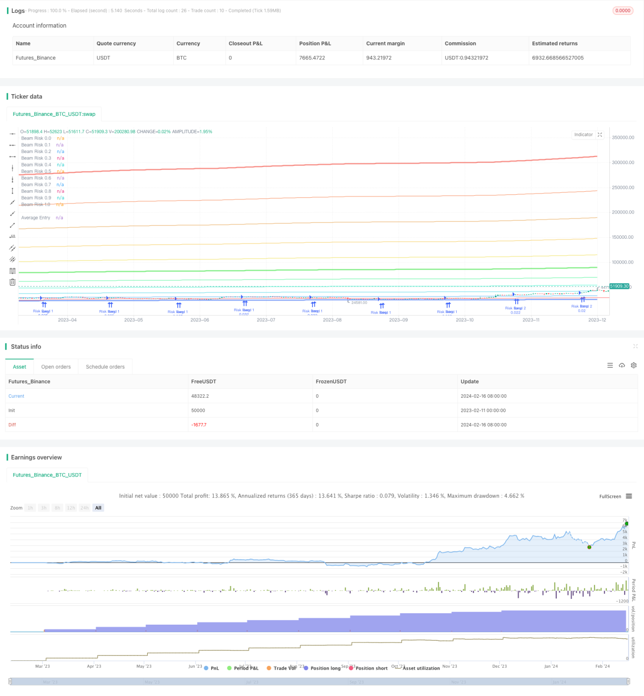
/*backtest
start: 2023-02-11 00:00:00
end: 2024-02-17 00:00:00
period: 1d
basePeriod: 1h
exchanges: [{"eid":"Futures_Binance","currency":"BTC_USDT"}]
*/

// © gjfsdrtytru - BEAM DCA Strategy {
// Based on Ben Cowen's risk level strategy, this aims to copy that method but with BEAM band levels.
// Upper BEAM level is derived from ln(price/200W MA)/2.5, while the 200W MA is the floor price. This is our 0-1 range.
// Buy limit orders are set at the < 0.5 levels and sell orders are set at the > 0.5 level.- 1