Estrategia de múltiples factores

El autor:¿ Qué pasa?, Fecha: 2023-10-31 15:45:39
Las etiquetas:

Resumen general

La estrategia multifactorial integra las estrategias de oscilación, seguimiento de tendencias y ruptura en una sola al combinar sus fortalezas.

Estrategia lógica

La estrategia multifactorial se basa principalmente en los siguientes aspectos:

La parte oscilante utiliza el oscilador estocástico para identificar señales de compra y venta. Específicamente, se genera una señal de compra cuando la línea %K cruza la línea %D desde la zona de sobreventa. Se genera una señal de venta cuando la línea %K cruza por debajo de la línea %D desde la zona de sobrecompra.
La parte que sigue la tendencia utiliza la cruz de oro de las SMA para determinar la dirección de la tendencia. Una señal de compra se genera cuando la SMA rápida cruza por encima de la SMA lenta. Una señal de venta se genera cuando la SMA rápida cruza por debajo de la SMA lenta.
La parte de ruptura monitorea si el precio se rompe por encima del precio más alto o se rompe por debajo del precio más bajo en un período especificado.
El indicador ADX se utiliza para medir la fuerza de la tendencia.
Las líneas de stop loss y take profit se implementan para optimizar la rentabilidad.

En resumen, la estrategia multifactorial sigue la lógica siguiente:

Cuando el ADX está por encima de un umbral, la tendencia se considera fuerte. La estrategia de seguimiento de tendencia tiene efecto. Cuando el ADX está por debajo del umbral, el mercado está variando. Solo la estrategia oscilante tiene efecto.
En un mercado de tendencia, la cruz de oro de la SMA desencadena una entrada larga y la cruz de muerte desencadena posiciones de salida.
En un mercado variante, se siguen las señales de negociación del oscilador estocástico.
La estrategia de ruptura se aplica en ambas condiciones de mercado para seguir un fuerte impulso.
Las líneas de stop loss y take profit están configuradas para bloquear las ganancias y limitar las pérdidas.

Análisis de ventajas

La mayor ventaja de la estrategia multifactorial es que combina las fortalezas de diferentes estrategias y consigue un buen rendimiento tanto en los mercados de tendencia como en los de variación.

Conduce bien las tendencias y logra altas tasas de ganancia en los mercados de tendencia.
Puede beneficiarse de los mercados de rango y evitar quedarse atascado en posiciones.
Tiene altos factores de ganancia con stop loss y take profit adecuadamente establecidos.
Considera la fuerza de la tendencia para reducir las pérdidas por señales falsas.
La combinación de múltiples indicadores conduce a fuertes señales comerciales.
Los parámetros se pueden optimizar para un mejor rendimiento.

Análisis de riesgos

También existen riesgos asociados con la estrategia multifactorial:

Una combinación incorrecta de factores puede dar lugar a señales comerciales contradictorias.
Los múltiples parámetros aumentan la dificultad de la optimización y requieren datos históricos suficientes.
Es posible que no pueda salir de las posiciones a tiempo cuando la tendencia se invierta, lo que conduce a grandes pérdidas.
El indicador ADX tiene efectos de retraso y puede perder los puntos de inflexión de la tendencia.
El comercio de breakout es propenso a quedar atrapado en posiciones perdedoras.

Los riesgos pueden mitigarse mediante:

Prueba de la estabilidad de los factores y selección de los estables.
Usando algoritmos de optimización heurística para encontrar los parámetros óptimos.
Configurar el stop loss adecuado para controlar el descenso máximo.
Incorporación de indicadores adicionales para detectar la reversión de tendencia.
Optimización de las reglas de stop loss para el comercio de ruptura.

Direcciones de mejora

La estrategia de múltiples factores aún puede mejorarse:

Probando más tipos de factores como volatilidad, volumen, etc. para encontrar mejores combinaciones.
Usando técnicas de aprendizaje automático para optimizar los factores de peso dinámicamente.
Aprovechando algoritmos heurísticos para la optimización rápida de parámetros.
Prueba de la rentabilidad en diferentes períodos de tenencia.
Explorar reglas dinámicas de stop loss, por ejemplo, ampliar el stop loss después de obtener algunas ganancias.
Añadir más filtros como picos de volumen para mejorar la calidad de la señal.
Optimización de los parámetros ADX o uso de indicadores de detección de tendencias más avanzados.

Conclusión

La estrategia multifactor combina múltiples lógicas de negociación como tendencia, reversión media y ruptura. Se logra un buen rendimiento tanto en mercados de tendencia como de rango. En comparación con las estrategias de un solo factor, proporciona rendimientos más estables y tiene un gran potencial para actualizaciones. Sin embargo, la optimización de parámetros podría ser difícil y requiere suficientes datos históricos. En general, la estrategia multifactor es una técnica de negociación algorítmica muy efectiva que vale la pena investigar y optimizar más.

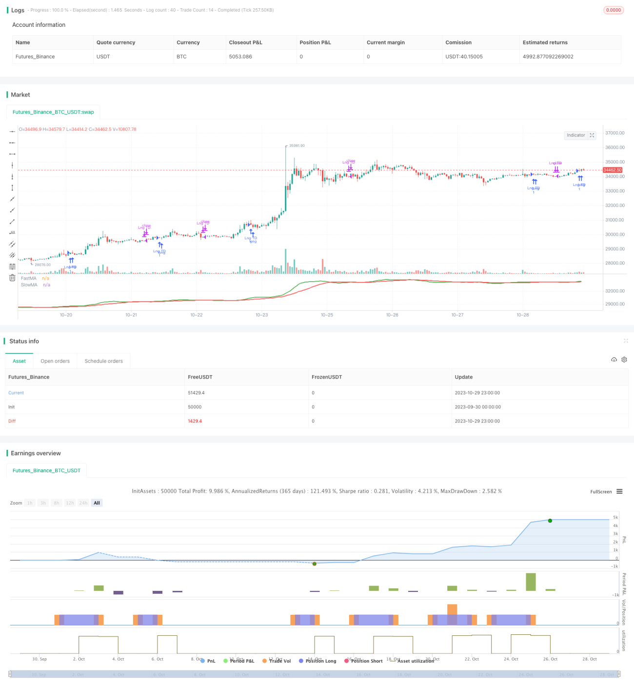
/*backtest
start: 2023-09-30 00:00:00
end: 2023-10-30 00:00:00
period: 1h
basePeriod: 15m
exchanges: [{"eid":"Futures_Binance","currency":"BTC_USDT"}]
*/

//@version=4

// strategy("Strategy_1", shorttitle="Strategy1",overlay=true ,pyramiding = 12, initial_capital=25000, currency='EUR', commission_type = strategy.commission.cash_per_order, commission_value = 3, default_qty_type = strategy.percent_of_equity, default_qty_value = 20)
	
// Revision:        1
// Author:          Jonas

// === INPUT ===
    //   > BACKTEST RANGE <
FromMonth = input(defval=1, title="From Month", minval=1, maxval=12)
FromDay = input(defval=1, title="From Day", minval=1, maxval=31)
FromYear = input(defval=2017, title="From Year", minval=2010)
ToMonth = input(defval=1, title="To Month", minval=1, maxval=12)
ToDay = input(defval=1, title="To Day", minval=1, maxval=31)
ToYear = input(defval=9999, title="To Year", minval=2010)

    //   > STRATEGY SETTINGS <
bolOS = input(defval = false, type=input.bool, title="Oscillating Strategy")
bolTS = input(defval = true, type=input.bool, title="Trend Strategy")
bolBO = input(defval = false, type=input.bool, title="Breakout Strategy")

strStrategy = input(defval = "Long", type=input.string, title="Trade Strategy",options = ["Long", "Short","Long & Short"])

flStopLoss = input(defval = 2.0, title="Stop Loss %", type=input.float)/100
flTakeProfit = input(defval = 4.0, title="Take Profit %", type=input.float)/100

    //   > SMA <

fastMA = input(defval=8, type=input.integer, title="FastMA length", minval=1, step=1)
slowMA = input(defval=21, type=input.integer, title="SlowMA length", minval=1, step=1)

    //  > ADX <
adx_len = input(defval=10, type=input.integer, title="ADX length", minval=1, step=1)
adx_trend = input(defval=30, type=input.integer, title="ADX Tr", minval=1, step=1)
adx_choppy = adx_trend
adx_limit = adx_trend

    //  > TRENDSCORE <
ts_fromIndex = input(title="From", type=input.integer, minval=1, defval=10)
ts_toIndex = input(title="To", type=input.integer, minval=1, defval=14)
ts_src = input(title="Source", type=input.source, defval=close)

    // > Oscillator <
stoch_length = 14
stoch_OverBought = 75
stoch_OverSold = 25
stoch_smoothK = 3
stoch_smoothD = 3

// === BACK TEST RANGE FUNCTION ===
window_start = timestamp(FromYear, FromMonth, FromDay, 00, 00)  // backtest start window
window_finish = timestamp(ToYear, ToMonth, ToDay, 23, 59)  // backtest finish window
window() =>  // create function "within window of time"
    time >= window_start and time <= window_finish ? true : false

//plot(stop_level_Long, title="TEST",color=color.red, style=plot.style_linebr, linewidth=2)
//plot(take_level_Long, color=color.green, style=plot.style_linebr, linewidth=2)

// === ADX ===
adx_up = change(high)
adx_down = -change(low)
adx_trur = rma(tr, adx_len)
adx_plus = fixnan(100 * rma(adx_up > adx_down and adx_up > 0 ? adx_up : 0, adx_len) / adx_trur)
adx_minus = fixnan(100 * rma(adx_down > adx_up and adx_down > 0 ? adx_down : 0, adx_len) / adx_trur)
adx_sum = adx_plus + adx_minus

ADX = 100 * rma(abs(adx_plus - adx_minus) / (adx_sum == 0 ? 1 : adx_sum), adx_len)

//=== TRENDSCORE ===
trendscore(ts_src, ts_fromIndex, ts_toIndex) =>
	ts_sum = 0.0
	for i = ts_fromIndex to ts_toIndex
        ts_sum := ts_sum + (ts_src >= nz(ts_src[i]) ? 1 : -1)
    ts_sum

intTS = trendscore(ts_src, ts_fromIndex, ts_toIndex)
// Long if  TrendDirection = 1, Short if TrendDirection = -1; Indifferent if TrendDirection = 0
intTrendDirection = (intTS > (ts_toIndex-ts_fromIndex)) ? 1 : (intTS < (ts_fromIndex-ts_toIndex)) ? -1 : 0

    //  > TREND CONDITION <
adx_growing = ADX > highest(ADX[1],3)
intTrend = ((ADX >= adx_limit) and (ADX[1] >= adx_limit) and adx_growing) ? intTrendDirection : 0

// === ATR ===
ATR = sma(tr,10)
ATR_100 = ATR /abs(high - low)


// === STOCHASTICS ===

stoch_k = sma(stoch(close, high, low, stoch_length), stoch_smoothK)
stoch_d = sma(stoch_k, stoch_smoothD)

// === FILTER & CONDITIONS ===
    //  > STOCHASTICS <
bolFilter_OS1 = close[1] > hl2[1]



bolSigOsc_long_1 = (na(stoch_k) or na(stoch_d)) ? false : (crossover(stoch_d,stoch_OverSold) and stoch_k > stoch_d) ? true:false
bolSigOsc_short_1 = (na(stoch_k) or na(stoch_d)) ? false : (crossunder(stoch_d,stoch_OverBought) and stoch_k < stoch_d) ? true:false

bolLongOpenOS = bolSigOsc_long_1 and bolFilter_OS1
bolLongCloseOS = bolSigOsc_short_1

bolShortOpenOS = bolSigOsc_short_1 and bolFilter_OS1
bolShortCloseOS = bolSigOsc_long_1

    //  > TREND <

bolFilter_TS1 = close[1] > hl2[1] and open[1] < hl2[1]
bolFilter_TS2 = sma(close,50)>sma(close,50)[10]
bolFilter_TS3 = close[1] < hl2[1] and open[1] > hl2[1]

bolSigTrendLO1 = sma(close, fastMA) > sma(close, slowMA)
bolSigTrendLO2 = close > sma(close,fastMA)
bolSigTrendLO3 = bolSigTrendLO1 and bolSigTrendLO2

bolSigTrendLC1 = sma(close, fastMA) < sma(close, slowMA)
bolSigTrendLC2 = close < sma(close, fastMA)
bolSigTrendLC3 = bolSigTrendLC1 and bolSigTrendLC2

bolSigTrendSO1 = bolSigTrendLC3
bolSigTrendSC1 = bolSigTrendLO1

bolLongOpenTS = bolSigTrendLO3 and bolFilter_TS1
bolLongCloseTS = bolSigTrendLC3 and bolFilter_TS3

bolShortOpenTS = bolSigTrendSO1 and bolFilter_TS3
bolShortCloseTS = bolLongOpenTS and bolFilter_TS1

plot(sma(close, fastMA), title='FastMA', color=color.green, linewidth=2, style=plot.style_line)  // plot FastMA
plot(sma(close, slowMA), title='SlowMA', color=color.red, linewidth=2, style=plot.style_line)  // plot SlowMA



    //  > BREAKOUT <
flFilter_BS1 = 0.5 * stdev(close,slowMA)[1]
bolFilter_BS2 = volume > sma(volume,slowMA)*1.25

bolSigBreakoutLO1 = close > (highestbars(high,slowMA)[1] + flFilter_BS1)
bolSigBreakoutLC1 = barssince(bolSigBreakoutLO1)==5

bolSigBreakoutSO1 = close < lowestbars(low,slowMA)[1] - flFilter_BS1
bolSigBreakoutSC1 = barssince(bolSigBreakoutSO1)==5


bolLongOpenBO = bolSigBreakoutLO1 and bolFilter_BS2
bolLongCloseBO = bolSigBreakoutLC1

bolShortOpenBO = bolSigBreakoutSO1 and bolFilter_BS2
bolShortCloseBO = bolSigBreakoutSC1

//=== STRATEGIES ENTRIES & EXITS ===
    //  > STOPS & LIMITS <
stop_level_Long = strategy.position_avg_price * (1 - flStopLoss)
take_level_Long = strategy.position_avg_price * (1 + flTakeProfit)
stop_level_Short = strategy.position_avg_price * (1 + flStopLoss)
take_level_Short = strategy.position_avg_price * (1 - flTakeProfit)

    //  > ENTRIES / CLOSES / EXITS <
if window() //only in backtest-window
    if (bolOS == true)
        if (intTrend == 0)
            if(strStrategy == "Long" or strStrategy == "Long & Short")
                strategy.entry("Lng Osc", strategy.long, when=bolLongOpenOS)  // buy long when "within window of time" AND crossover
            if(strStrategy == "Short" or strStrategy == "Long & Short")
                strategy.entry("Short Osc", strategy.short, when=bolShortOpenOS)
        strategy.close("Lng Osc", when=(bolLongCloseOS))
        //strategy.exit("Exit L OS/STD", "Lng Osc", stop = strategy.position_avg_price - 2*stdev(close,10))
        strategy.exit("Exit L OS/%", "Lng Osc", stop=stop_level_Long)
        strategy.close("Short Osc", when=(bolShortCloseOS))
        //strategy.exit("Exit S OS/STD", "Short Osc", stop = strategy.position_avg_price + 2*stdev(strategy.position_avg_price,10))
        strategy.exit("Exit S OS/%", "Short Osc", stop=stop_level_Short)
    if (bolTS == true)
        if (not(intTrend == 0))
            if((strStrategy == "Long") or (strStrategy == "Long & Short"))
                strategy.entry("Lng TD", strategy.long, when=bolLongOpenTS)  // buy long when "within window of time" AND crossover
            if((strStrategy == "Short") or (strStrategy == "Long & Short"))
                strategy.entry("Short TD", strategy.short, when=(bolShortOpenTS and bolTS))  // buy long when "within window of time" AND crossover
        strategy.exit("Exit L TD", "Lng TD", stop=stop_level_Long)
        strategy.close("Lng TD", when=bolLongCloseTS)
        strategy.exit("Exit S TD", "Short TD", stop=stop_level_Short)
        strategy.close("Short TD", when=bolShortCloseTS)
    if (bolBO == true)
        if((strStrategy == "Long") or (strStrategy == "Long & Short"))
            strategy.entry("Lng BO", strategy.long, when=bolLongOpenBO)  // buy long when "within window of time" AND crossover
            strategy.close("Lng BO", when=bolLongCloseBO)
            //strategy.exit("Exit L BO/STD", "Lng BO", stop = strategy.position_avg_price - 2*stdev(strategy.position_avg_price,10))
            strategy.exit("Exit L BO/2.5%", "Lng BO", stop=stop_level_Long)
        if((strStrategy == "Short") or (strStrategy == "Long & Short"))
            strategy.entry("Short BO", strategy.short, when=bolShortOpenBO)  // buy long when "within window of time" AND crossover
            strategy.close("Short BO", when=bolShortCloseBO)
            //strategy.exit("Exit S BO/STD", "Short BO", stop = strategy.position_avg_price - 2*stdev(strategy.position_avg_price,10))
            strategy.exit("Exit S BO/%", "Short BO", stop=stop_level_Short)

Más.