Estrategia de cruce de media móvil ponderada por impulso y media móvil doble
Descripción general
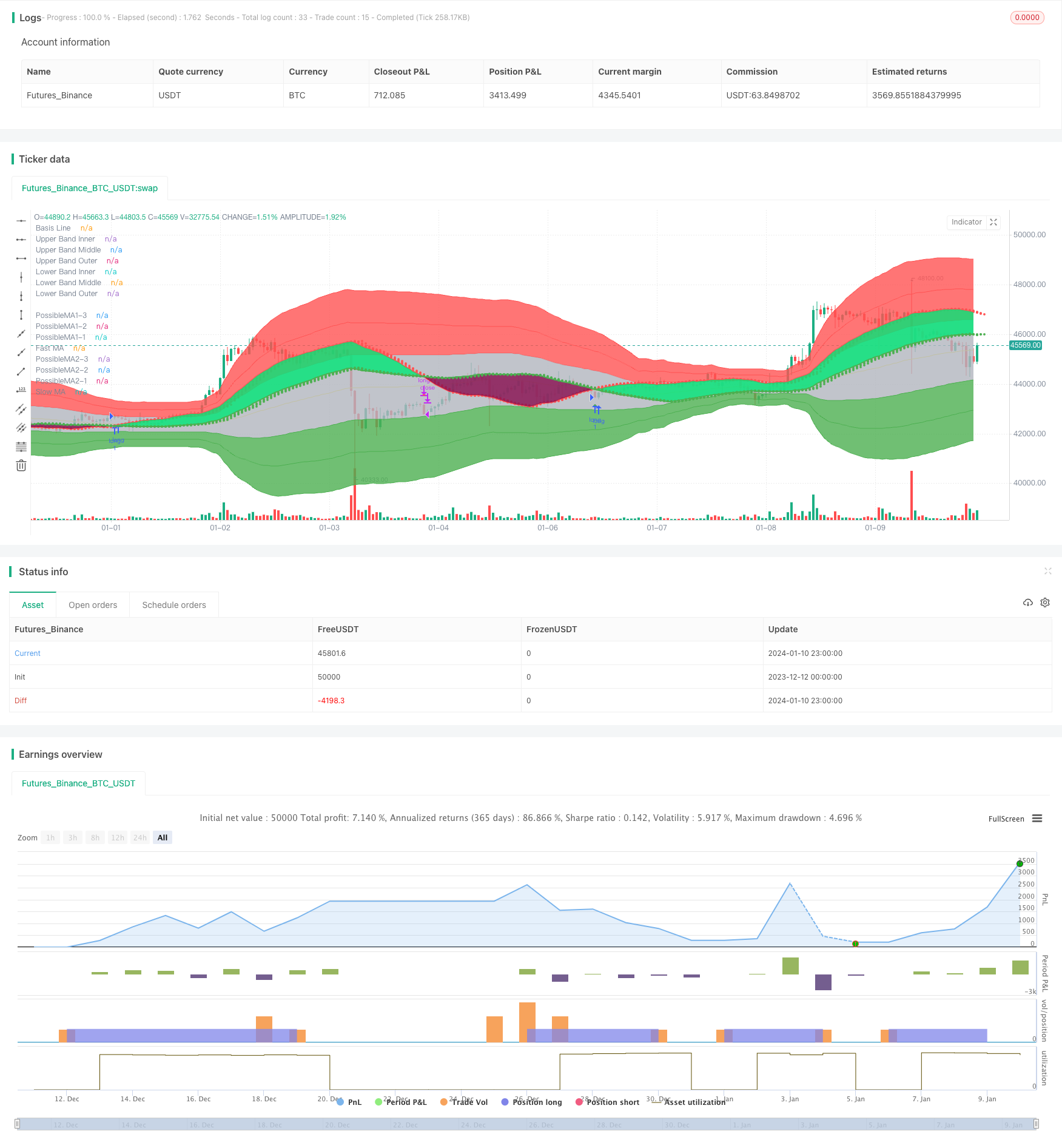
La estrategia genera señales de compra y venta cuando se cruzan mediante el cálculo de dos promedios móviles ponderados por la energía (MAEMA) de dos períodos diferentes. La línea de corto período se utiliza para determinar las tendencias del mercado y las señales de reversión a corto plazo, mientras que la línea de largo período se utiliza para determinar la dirección de la tendencia principal.
El principio
- Calcula el MAEMA de la línea rápida (80 ciclos) y la línea lenta (-144 ciclos).
- Las líneas rápidas reflejan las tendencias a corto plazo y los puntos de inflexión. Las líneas lentas reflejan la dirección de las tendencias principales.
- Cuando la línea rápida atraviesa la línea lenta, genera una señal de compra. Cuando la línea rápida atraviesa la línea lenta, genera una señal de venta.
- La estrategia traza simultáneamente 3 puntos de pronóstico que representan los valores probables para el siguiente ciclo, para así juzgar las tendencias cruzadas en el futuro.
- La estrategia aprovecha al máximo la dinámica y la capacidad de predicción del propio indicador MAEMA.
Análisis de las ventajas
- El MAEMA, por su parte, integra un factor de dinámica para captar más rápidamente los cambios en las tendencias.
- Estrategias de doble línea para determinar la dirección de las tendencias en diferentes períodos de tiempo.
- La combinación de la intersección de las líneas rápidas y lentas con los propios puntos de predicción de MAEMA hace que las señales de compra y venta sean más fiables.
- El mapa automático es completo y refleja las fluctuaciones del mercado de forma intuitiva.
Análisis de riesgos
- En caso de fluctuaciones anormales en el mercado, la sensibilidad del indicador MAEMA puede ser demasiado alta y generar una señal errónea. Se puede relajar adecuadamente el punto de parada.
- El sistema de línea media es propenso a generar falsas señales para el mercado horizontal. Se pueden agregar otros filtros.
- La configuración periódica de las líneas rápidas y lentas requiere determinar los parámetros óptimos según las diferentes variedades.
Dirección de optimización
- Optimización de los parámetros de periodicidad de las líneas rápidas y lentas de MAEMA para encontrar la combinación óptima de parámetros.
- Aumentar las condiciones de filtración para evitar la apertura de posiciones en situaciones de crisis. Por ejemplo, la introducción de DMI, MACD y otras tendencias de juicio.
- Ajuste continuamente el coeficiente ATR de acuerdo con los resultados de las pruebas de retroalimentación y mueva el punto de parada para reducir los falsos positivos y controlar el riesgo.
Resumir
La estrategia utiliza el movimiento de la energía ponderada de las medias móviles para determinar los cambios en la tendencia del mercado, los principios básicos son claros y simples. En combinación con la propia dinámica de MAEMA y la función de predicción, la identificación de las señales de reversión es más eficaz. Se debe prestar atención a la optimización de los parámetros y el fortalecimiento de las condiciones de filtración para mejorar la estabilidad.
/*backtest
start: 2023-12-12 00:00:00
end: 2024-01-11 00:00:00
period: 1h
basePeriod: 15m
exchanges: [{"eid":"Futures_Binance","currency":"BTC_USDT"}]
*/

// © informanerd
//@version=4

strategy("MultiType Shifting Predictive MAs Crossover", shorttitle = "MTSPMAC + MBHB Strategy", overlay = true)

//inputs

predict = input(true, "Show MA Prediction Tails")
trendFill = input(true, "Fill Between MAs Based on Trend")
signal = input(true, "Show Cross Direction Signals")

showMA1 = input(true, "[ Show Fast Moving Average ]══════════")
type1 = input("MAEMA (Momentum Adjusted Exponential)", "Fast MA Type", options = ["MAEMA (Momentum Adjusted Exponential)", "DEMA (Double Exponential)", "EMA (Exponential)", "HMA (Hull)", "LSMA (Least Squares)", "RMA (Adjusted Exponential)", "SMA (Simple)", "SWMA (Symmetrically Weighted)", "TEMA (Triple Exponential)", "TMA (Triangular)", "VMA / VIDYA (Variable Index Dynamic Average)", "VWMA (Volume Weighted)", "WMA (Weighted)"])
src1 = input(high, "Fast MA Source")
len1 = input(80, "Fast MA Length", minval = 2)
shift1 = input(0, "Fast MA Shift")
maThickness1 = input(2, "Fast MA Thickness", minval = 1)
trendColor1 = input(false, "Color Fast MA Based on Detected Trend")
showBand1 = input(false, "Show Fast MA Range Band")
atrPer1 = input(20, "Fast Band ATR Lookback Period")
atrMult1 = input(3, "Fast Band ATR Multiplier")

showMA2 = input(true, "[ Show Slow Moving Average ]══════════")
type2 = input("MAEMA (Momentum Adjusted Exponential)", "Slow MA Type", options = ["MAEMA (Momentum Adjusted Exponential)", "DEMA (Double Exponential)", "EMA (Exponential)", "HMA (Hull)", "LSMA (Least Squares)", "RMA (Adjusted Exponential)", "SMA (Simple)", "SWMA (Symmetrically Weighted)", "TEMA (Triple Exponential)", "TMA (Triangular)", "VMA / VIDYA (Variable Index Dynamic Average)", "VWMA (Volume Weighted)", "WMA (Weighted)"])
src2 = input(close, "Slow MA Source")
len2 = input(144, "Slow MA Length", minval = 2)
shift2 = input(0, "Slow MA Shift")
maThickness2 = input(2, "Slow MA Thickness", minval = 1)
trendColor2 = input(false, "Color Slow MA Based on Detected Trend")
showBand2 = input(false, "Show Slow MA Range Band")
atrPer2 = input(20, "Slow Band ATR Lookback Period")
atrMult2 = input(3, "Slow Band ATR Multiplier")

//ma calculations

ma(type, src, len) =>
    if type == "MAEMA (Momentum Adjusted Exponential)"
        goldenRatio = (1 + sqrt(5)) / 2
        momentumLen = round(len / goldenRatio), momentum = change(src, momentumLen), probabilityLen = len / goldenRatio / goldenRatio
        ema(src + (momentum + change(momentum, momentumLen) * 0.5) * sum(change(src) > 0 ? 1 : 0, round(probabilityLen)) / probabilityLen, len)
    else if type == "DEMA (Double Exponential)"
        2 * ema(src, len) - ema(ema(src, len), len)
    else if type == "EMA (Exponential)"
        ema(src, len)
    else if type == "HMA (Hull)"
        wma(2 * wma(src, len / 2) - wma(src, len), round(sqrt(len)))
    else if type == "LSMA (Least Squares)"
        3 * wma(src, len) - 2 * sma(src, len)
    else if type == "RMA (Adjusted Exponential)"
        rma(src, len)
    else if type == "SMA (Simple)"
        sma(src, len)
    else if type == "SWMA (Symmetrically Weighted)"
        swma(src)
    else if type == "TEMA (Triple Exponential)"
        3 * ema(src, len) - 3 * ema(ema(src, len), len) + ema(ema(ema(src, len), len), len)
    else if type == "TMA (Triangular)"
        swma(wma(src, len))
    else if type == "VMA / VIDYA (Variable Index Dynamic Average)"
        smoothing = 2 / len, volIndex = abs(cmo(src, len) / 100)
        vma = 0., vma := (smoothing * volIndex * src) + (1 - smoothing * volIndex) * nz(vma[1])
    else if type == "VWMA (Volume Weighted)"
        vwma(src, len)
    else if type == "WMA (Weighted)"
        wma(src, len)

ma1 = ma(type1, src1, len1)
ma2 = ma(type2, src2, len2)

//ma predictions

pma11 = len1 > 2 ? (ma(type1, src1, len1 - 1) * (len1 - 1) + src1 * 1) / len1 : na
pma12 = len1 > 3 ? (ma(type1, src1, len1 - 2) * (len1 - 2) + src1 * 2) / len1 : na
pma13 = len1 > 4 ? (ma(type1, src1, len1 - 3) * (len1 - 3) + src1 * 3) / len1 : na

pma21 = len2 > 2 ? (ma(type2, src2, len2 - 1) * (len2 - 1) + src2 * 1) / len2 : na
pma22 = len2 > 3 ? (ma(type2, src2, len2 - 2) * (len2 - 2) + src2 * 2) / len2 : na
pma23 = len2 > 4 ? (ma(type2, src2, len2 - 3) * (len2 - 3) + src2 * 3) / len2 : na

//ma range bands

r1 = atr(atrPer1) * atrMult1
hBand1 = ma1 + r1
lBand1 = ma1 - r1

r2 = atr(atrPer2) * atrMult2
hBand2 = ma2 + r2
lBand2 = ma2 - r2

//drawings

ma1Plot = plot(showMA1 ? ma1 : na, "Fast MA", trendColor1 and ma1 > src1 ? color.maroon : trendColor1 and ma1 < src1 ? color.lime : trendColor1 ? color.gray : color.red, maThickness1, offset = shift1)
ma2Plot = plot(showMA2 ? ma2 : na, "Slow MA", trendColor2 and ma2 > src2 ? color.maroon : trendColor2 and ma2 < src2 ? color.lime : trendColor2 ? color.gray : color.green, maThickness2, offset = shift2)
fill(ma1Plot, ma2Plot, trendFill and ma1 > ma2 ? color.lime : trendFill and ma1 < ma2 ? color.maroon : na, 90)

plot(showMA1 and predict ? pma11 : na, "PossibleMA1-1", trendColor1 and ma1 > src1 ? color.maroon : trendColor1 and ma1 < src1 ? color.lime : trendColor1 ? color.gray : color.red, style = plot.style_circles, offset = shift1 + 1, show_last = 1)
plot(showMA1 and predict ? pma12 : na, "PossibleMA1-2", trendColor1 and ma1 > src1 ? color.maroon : trendColor1 and ma1 < src1 ? color.lime : trendColor1 ? color.gray : color.red, style = plot.style_circles, offset = shift1 + 2, show_last = 1)
plot(showMA1 and predict ? pma13 : na, "PossibleMA1-3", trendColor1 and ma1 > src1 ? color.maroon : trendColor1 and ma1 < src1 ? color.lime : trendColor1 ? color.gray : color.red, style = plot.style_circles, offset = shift1 + 3, show_last = 1)
plot(showMA2 and predict ? pma21 : na, "PossibleMA2-1", trendColor2 and ma2 > src2 ? color.maroon : trendColor2 and ma2 < src2 ? color.lime : trendColor2 ? color.gray : color.green, style = plot.style_circles, offset = shift2 + 1, show_last = 1)
plot(showMA2 and predict ? pma22 : na, "PossibleMA2-2", trendColor2 and ma2 > src2 ? color.maroon : trendColor2 and ma2 < src2 ? color.lime : trendColor2 ? color.gray : color.green, style = plot.style_circles, offset = shift2 + 2, show_last = 1)
plot(showMA2 and predict ? pma23 : na, "PossibleMA2-3", trendColor2 and ma2 > src2 ? color.maroon : trendColor2 and ma2 < src2 ? color.lime : trendColor2 ? color.gray : color.green, style = plot.style_circles, offset = shift2 + 3, show_last = 1)

plot(showBand1 ? hBand1 : na, "Fast Higher Band", trendColor1 and ma1 > src1 ? color.maroon : trendColor1 and ma1 < src1 ? color.lime : trendColor1 ? color.gray : color.red, offset = shift1)
plot(showBand1 ? lBand1 : na, "Fast Lower Band", trendColor1 and ma1 > src1 ? color.maroon : trendColor1 and ma1 < src1 ? color.lime : trendColor1 ? color.gray : color.red, offset = shift1)
plot(showBand2 ? hBand2 : na, "Slow Higher Band", trendColor2 and ma2 > src2 ? color.maroon : trendColor2 and ma2 < src2 ? color.lime : trendColor2 ? color.gray : color.green, offset = shift2)
plot(showBand2 ? lBand2 : na, "Slow Lower Band", trendColor2 and ma2 > src2 ? color.maroon : trendColor2 and ma2 < src2 ? color.lime : trendColor2 ? color.gray : color.green, offset = shift2)

//crosses & alerts

up = crossover(ma1, ma2)
down = crossover(ma2, ma1)

plotshape(signal ? up : na, "Buy", shape.triangleup, location.belowbar, color.green, offset = shift1, size = size.small)
plotshape(signal ? down : na, "Sell", shape.triangledown, location.abovebar, color.red, offset = shift1, size = size.small)

alertcondition(up, "Buy", "Buy")
alertcondition(down, "Sell", "Sell")

// @version=1

// Title: "Multi Bollinger Heat Bands - EMA/Breakout options".
// Author: JayRogers
//
// * Description *
//   Short: It's your Basic Bollinger Bands, but 3 of them, and some pointy things.
//
//   Long:  Three stacked sma based Bollinger Bands designed just to give you a quick visual on the "heat" of movement.
//          Set inner band as you would expect, then set your preferred additional multiplier increments for the outer 2 bands.
//          Option to use EMA as alternative basis, rather than SMA.
//          Breakout indication shapes, which have their own multiplier seperate from the BB's; but still tied to same length/period.

// strategy(shorttitle="[JR]MBHB_EBO", title="[JR] Multi Bollinger Heat Bands - EMA/Breakout options", overlay=true)

// Bollinger Bands Inputs
bb_use_ema = input(false, title="Use EMA Basis?")
bb_length = input(80, minval=1, title="Bollinger Length")
bb_source = input(close, title="Bollinger Source")
bb_mult = input(1.0, title="Base Multiplier", minval=0.001, maxval=50)
bb_mult_inc = input(1, title="Multiplier Increment", minval=0.001, maxval=2)
// Breakout Indicator Inputs
break_mult = input(3, title="Breakout Multiplier", minval=0.001, maxval=50)
breakhigh_source = input(high, title="High Break Source")
breaklow_source = input(low, title="Low Break Source")

bb_basis = bb_use_ema ? ema(bb_source, bb_length) : sma(bb_source, bb_length)

// Deviation
// * I'm sure there's a way I could write some of this cleaner, but meh.
dev = stdev(bb_source, bb_length)
bb_dev_inner = bb_mult * dev
bb_dev_mid = (bb_mult + bb_mult_inc) * dev
bb_dev_outer = (bb_mult + (bb_mult_inc * 2)) * dev
break_dev = break_mult * dev

// Upper bands
inner_high = bb_basis + bb_dev_inner
mid_high = bb_basis + bb_dev_mid
outer_high = bb_basis + bb_dev_outer
// Lower Bands
inner_low = bb_basis - bb_dev_inner
mid_low = bb_basis - bb_dev_mid
outer_low = bb_basis - bb_dev_outer

// Breakout Deviation
break_high = bb_basis + break_dev
break_low = bb_basis - break_dev

// plot basis
plot(bb_basis, title="Basis Line", color=color.yellow, transp=50)

// plot and fill upper bands
ubi = plot(inner_high, title="Upper Band Inner", color=color.red, transp=90)
ubm = plot(mid_high, title="Upper Band Middle", color=color.red, transp=85)
ubo = plot(outer_high, title="Upper Band Outer", color=color.red, transp=80)
fill(ubi, ubm, title="Upper Bands Inner Fill", color=color.red, transp=90)
fill(ubm, ubo, title="Upper Bands Outer Fill",color=color.red, transp=80)

// plot and fill lower bands
lbi = plot(inner_low, title="Lower Band Inner", color=color.green, transp=90)
lbm = plot(mid_low, title="Lower Band Middle", color=color.green, transp=85)
lbo = plot(outer_low, title="Lower Band Outer", color=color.green, transp=80)
fill(lbi, lbm, title="Lower Bands Inner Fill", color=color.green, transp=90)
fill(lbm, lbo, title="Lower Bands Outer Fill", color=color.green, transp=80)

// center channel fill
fill(ubi, lbi, title="Center Channel Fill", color=color.silver, transp=100)

// plot breakouts
plotshape(breakhigh_source >= break_high, title="High Breakout", style=shape.triangledown, location=location.abovebar, size=size.tiny, color=color.white, transp=0)
plotshape(breaklow_source <= break_low, title="Low Breakout", style=shape.triangleup, location=location.belowbar, size=size.tiny, color=color.white, transp=0)
High_Break = breakhigh_source >= break_high
Low_Break = breaklow_source <= break_low

// Conditions
Stop_Momentum = low < ma1

//Strategy Tester

strategy.entry("long", strategy.long, when=(up and (hlc3 < inner_high)))
strategy.close("long", when=down)

strategy.entry("longwickdown", strategy.long, when=Low_Break)
strategy.close("longwickdown", when=(high > ma1))

//true signals test

//var winCount = 0, var loseCount = 0, testBarIndex = 1
//if (up[testBarIndex] and close > close[testBarIndex]) or (down[testBarIndex] and close < close[testBarIndex])
//    label.new(bar_index, 0, "W", yloc = yloc.abovebar, color = color.green)
//    winCount := winCount + 1
//else if (up[testBarIndex] and close < close[testBarIndex]) or (down[testBarIndex] and close > close[testBarIndex])
//    label.new(bar_index, 0, "L", yloc = yloc.abovebar, color = color.red)
//    loseCount := loseCount + 1
//winRate = label.new(time + (time - time[1]) * 2, ohlc4, tostring(round(winCount / (winCount + loseCount) * 100)) + "%", xloc = xloc.bar_time, color = color.orange, style = label.style_label_left)
//if not na(winRate[1])
//    label.delete(winRate[1])