Stratégie à facteurs multiples

Auteur:ChaoZhang est là., Date: le 31 octobre 2023 à 15h45
Les étiquettes:

Résumé

La stratégie multifactorielle intègre les stratégies d'oscillation, de suivi des tendances et de rupture en une seule en combinant leurs forces.

La logique de la stratégie

La stratégie multifactorielle est principalement modélisée sur la base des aspects suivants:

La partie oscillante utilise l'oscillateur stochastique pour identifier les signaux d'achat et de vente. Plus précisément, un signal d'achat est généré lorsque la ligne %K traverse la ligne %D de la zone de survente. Un signal de vente est généré lorsque la ligne %K traverse la ligne %D de la zone de surachat.
La partie suivant la tendance utilise la croix dorée des SMA pour déterminer la direction de la tendance. Un signal d'achat est généré lorsque la SMA rapide traverse au-dessus de la SMA lente. Un signal de vente est généré lorsque la SMA rapide traverse au-dessous de la SMA lente.
La partie de rupture surveille si le prix dépasse le prix le plus élevé ou tombe en dessous du prix le plus bas dans une période spécifiée.
L'indicateur ADX est utilisé pour mesurer la force de la tendance.
Les lignes de stop-loss et de prise de profit sont mises en œuvre pour optimiser la rentabilité.

En résumé, la stratégie multifactorielle suit la logique suivante:

Lorsque l'ADX est au-dessus d'un seuil, la tendance est considérée comme forte. La stratégie de suivi de la tendance prend effet. Lorsque l'ADX est en dessous du seuil, le marché varie. Seule la stratégie oscillante prend effet.
Dans un marché en tendance, la croix dorée de la SMA déclenche une entrée longue et la croix de la mort déclenche une sortie.
Dans un marché en variation, les signaux de négociation de l'oscillateur stochastique sont suivis.
La stratégie de rupture s'applique dans les deux conditions du marché pour suivre une dynamique forte.
Les lignes de stop loss et de take profit sont réglées pour verrouiller les bénéfices et limiter les pertes.

Analyse des avantages

L'avantage majeur de la stratégie multifactorielle est qu'elle combine les forces de différentes stratégies et réalise de bonnes performances sur les marchés tendance et variable.

Il suit bien les tendances et obtient des taux de réussite élevés sur les marchés en tendance.
Il peut tirer profit des marchés à plage et éviter de rester bloqué dans des positions.
Il a des facteurs de profit élevés avec un stop-loss et un take profit correctement réglés.
Il considère la force de la tendance pour réduire les pertes dues aux faux signaux.
La combinaison de plusieurs indicateurs conduit à des signaux de trading forts.
Les paramètres peuvent être optimisés pour une meilleure performance.

Analyse des risques

Il existe également des risques liés à la stratégie multifactorielle:

Une mauvaise combinaison de facteurs peut entraîner des signaux de trading contradictoires.
Les paramètres multiples augmentent la difficulté d'optimisation et nécessitent des données historiques suffisantes.
Il est possible qu'il ne parvienne pas à sortir de ses positions à temps lorsque la tendance s'inverse, ce qui entraînera des pertes importantes.
L'indicateur ADX a des effets de retard et peut manquer les points tournants de la tendance.
Le trading de rupture est enclin à se retrouver pris au piège dans des positions perdantes.

Les risques peuvent être atténués par:

Test de la stabilité des facteurs et sélection des facteurs stables.
Utiliser des algorithmes d'optimisation heuristique pour trouver les paramètres optimaux.
Réglage du stop-loss pour contrôler le maximum de tirage.
Incorporation d'indicateurs supplémentaires pour détecter un renversement de tendance.
Optimisation des règles de stop loss pour le trading de rupture.

Directions d'amélioration

La stratégie multifactorielle peut encore être améliorée:

Tester plus de types de facteurs comme la volatilité, le volume, etc. pour trouver de meilleures combinaisons.
Utiliser des techniques d'apprentissage automatique pour optimiser dynamiquement les poids des facteurs.
Utiliser des algorithmes heuristiques pour une optimisation rapide des paramètres.
Test de la rentabilité dans différentes périodes de détention.
Examiner les règles de stop loss dynamiques. Par exemple, élargir le stop loss après avoir réalisé des bénéfices.
Ajouter plus de filtres comme des pics de volume pour améliorer la qualité du signal.
Optimiser les paramètres ADX ou utiliser des indicateurs de détection de tendance plus avancés.

Conclusion

La stratégie multi-facteur combine plusieurs logiques de trading telles que la tendance, l'inversion moyenne et la rupture. Elle atteint de bonnes performances sur les marchés à la fois tendance et variable. Par rapport aux stratégies à facteur unique, elle offre des rendements plus stables et a un grand potentiel d'amélioration. Cependant, l'optimisation des paramètres peut être difficile et nécessite suffisamment de données historiques.

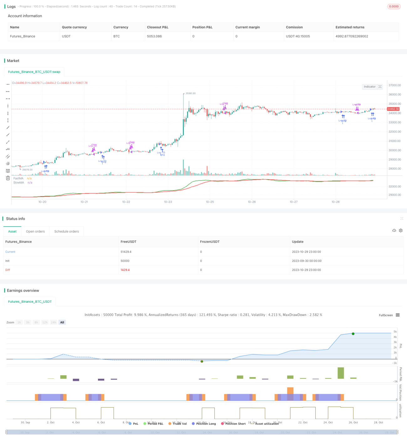
/*backtest
start: 2023-09-30 00:00:00
end: 2023-10-30 00:00:00
period: 1h
basePeriod: 15m
exchanges: [{"eid":"Futures_Binance","currency":"BTC_USDT"}]
*/

//@version=4

// strategy("Strategy_1", shorttitle="Strategy1",overlay=true ,pyramiding = 12, initial_capital=25000, currency='EUR', commission_type = strategy.commission.cash_per_order, commission_value = 3, default_qty_type = strategy.percent_of_equity, default_qty_value = 20)
	
// Revision:        1
// Author:          Jonas

// === INPUT ===
    //   > BACKTEST RANGE <
FromMonth = input(defval=1, title="From Month", minval=1, maxval=12)
FromDay = input(defval=1, title="From Day", minval=1, maxval=31)
FromYear = input(defval=2017, title="From Year", minval=2010)
ToMonth = input(defval=1, title="To Month", minval=1, maxval=12)
ToDay = input(defval=1, title="To Day", minval=1, maxval=31)
ToYear = input(defval=9999, title="To Year", minval=2010)

    //   > STRATEGY SETTINGS <
bolOS = input(defval = false, type=input.bool, title="Oscillating Strategy")
bolTS = input(defval = true, type=input.bool, title="Trend Strategy")
bolBO = input(defval = false, type=input.bool, title="Breakout Strategy")

strStrategy = input(defval = "Long", type=input.string, title="Trade Strategy",options = ["Long", "Short","Long & Short"])

flStopLoss = input(defval = 2.0, title="Stop Loss %", type=input.float)/100
flTakeProfit = input(defval = 4.0, title="Take Profit %", type=input.float)/100

    //   > SMA <

fastMA = input(defval=8, type=input.integer, title="FastMA length", minval=1, step=1)
slowMA = input(defval=21, type=input.integer, title="SlowMA length", minval=1, step=1)

    //  > ADX <
adx_len = input(defval=10, type=input.integer, title="ADX length", minval=1, step=1)
adx_trend = input(defval=30, type=input.integer, title="ADX Tr", minval=1, step=1)
adx_choppy = adx_trend
adx_limit = adx_trend

    //  > TRENDSCORE <
ts_fromIndex = input(title="From", type=input.integer, minval=1, defval=10)
ts_toIndex = input(title="To", type=input.integer, minval=1, defval=14)
ts_src = input(title="Source", type=input.source, defval=close)

    // > Oscillator <
stoch_length = 14
stoch_OverBought = 75
stoch_OverSold = 25
stoch_smoothK = 3
stoch_smoothD = 3

// === BACK TEST RANGE FUNCTION ===
window_start = timestamp(FromYear, FromMonth, FromDay, 00, 00)  // backtest start window
window_finish = timestamp(ToYear, ToMonth, ToDay, 23, 59)  // backtest finish window
window() =>  // create function "within window of time"
    time >= window_start and time <= window_finish ? true : false

//plot(stop_level_Long, title="TEST",color=color.red, style=plot.style_linebr, linewidth=2)
//plot(take_level_Long, color=color.green, style=plot.style_linebr, linewidth=2)

// === ADX ===
adx_up = change(high)
adx_down = -change(low)
adx_trur = rma(tr, adx_len)
adx_plus = fixnan(100 * rma(adx_up > adx_down and adx_up > 0 ? adx_up : 0, adx_len) / adx_trur)
adx_minus = fixnan(100 * rma(adx_down > adx_up and adx_down > 0 ? adx_down : 0, adx_len) / adx_trur)
adx_sum = adx_plus + adx_minus

ADX = 100 * rma(abs(adx_plus - adx_minus) / (adx_sum == 0 ? 1 : adx_sum), adx_len)

//=== TRENDSCORE ===
trendscore(ts_src, ts_fromIndex, ts_toIndex) =>
	ts_sum = 0.0
	for i = ts_fromIndex to ts_toIndex
        ts_sum := ts_sum + (ts_src >= nz(ts_src[i]) ? 1 : -1)
    ts_sum

intTS = trendscore(ts_src, ts_fromIndex, ts_toIndex)
// Long if  TrendDirection = 1, Short if TrendDirection = -1; Indifferent if TrendDirection = 0
intTrendDirection = (intTS > (ts_toIndex-ts_fromIndex)) ? 1 : (intTS < (ts_fromIndex-ts_toIndex)) ? -1 : 0

    //  > TREND CONDITION <
adx_growing = ADX > highest(ADX[1],3)
intTrend = ((ADX >= adx_limit) and (ADX[1] >= adx_limit) and adx_growing) ? intTrendDirection : 0

// === ATR ===
ATR = sma(tr,10)
ATR_100 = ATR /abs(high - low)


// === STOCHASTICS ===

stoch_k = sma(stoch(close, high, low, stoch_length), stoch_smoothK)
stoch_d = sma(stoch_k, stoch_smoothD)

// === FILTER & CONDITIONS ===
    //  > STOCHASTICS <
bolFilter_OS1 = close[1] > hl2[1]



bolSigOsc_long_1 = (na(stoch_k) or na(stoch_d)) ? false : (crossover(stoch_d,stoch_OverSold) and stoch_k > stoch_d) ? true:false
bolSigOsc_short_1 = (na(stoch_k) or na(stoch_d)) ? false : (crossunder(stoch_d,stoch_OverBought) and stoch_k < stoch_d) ? true:false

bolLongOpenOS = bolSigOsc_long_1 and bolFilter_OS1
bolLongCloseOS = bolSigOsc_short_1

bolShortOpenOS = bolSigOsc_short_1 and bolFilter_OS1
bolShortCloseOS = bolSigOsc_long_1

    //  > TREND <

bolFilter_TS1 = close[1] > hl2[1] and open[1] < hl2[1]
bolFilter_TS2 = sma(close,50)>sma(close,50)[10]
bolFilter_TS3 = close[1] < hl2[1] and open[1] > hl2[1]

bolSigTrendLO1 = sma(close, fastMA) > sma(close, slowMA)
bolSigTrendLO2 = close > sma(close,fastMA)
bolSigTrendLO3 = bolSigTrendLO1 and bolSigTrendLO2

bolSigTrendLC1 = sma(close, fastMA) < sma(close, slowMA)
bolSigTrendLC2 = close < sma(close, fastMA)
bolSigTrendLC3 = bolSigTrendLC1 and bolSigTrendLC2

bolSigTrendSO1 = bolSigTrendLC3
bolSigTrendSC1 = bolSigTrendLO1

bolLongOpenTS = bolSigTrendLO3 and bolFilter_TS1
bolLongCloseTS = bolSigTrendLC3 and bolFilter_TS3

bolShortOpenTS = bolSigTrendSO1 and bolFilter_TS3
bolShortCloseTS = bolLongOpenTS and bolFilter_TS1

plot(sma(close, fastMA), title='FastMA', color=color.green, linewidth=2, style=plot.style_line)  // plot FastMA
plot(sma(close, slowMA), title='SlowMA', color=color.red, linewidth=2, style=plot.style_line)  // plot SlowMA



    //  > BREAKOUT <
flFilter_BS1 = 0.5 * stdev(close,slowMA)[1]
bolFilter_BS2 = volume > sma(volume,slowMA)*1.25

bolSigBreakoutLO1 = close > (highestbars(high,slowMA)[1] + flFilter_BS1)
bolSigBreakoutLC1 = barssince(bolSigBreakoutLO1)==5

bolSigBreakoutSO1 = close < lowestbars(low,slowMA)[1] - flFilter_BS1
bolSigBreakoutSC1 = barssince(bolSigBreakoutSO1)==5


bolLongOpenBO = bolSigBreakoutLO1 and bolFilter_BS2
bolLongCloseBO = bolSigBreakoutLC1

bolShortOpenBO = bolSigBreakoutSO1 and bolFilter_BS2
bolShortCloseBO = bolSigBreakoutSC1

//=== STRATEGIES ENTRIES & EXITS ===
    //  > STOPS & LIMITS <
stop_level_Long = strategy.position_avg_price * (1 - flStopLoss)
take_level_Long = strategy.position_avg_price * (1 + flTakeProfit)
stop_level_Short = strategy.position_avg_price * (1 + flStopLoss)
take_level_Short = strategy.position_avg_price * (1 - flTakeProfit)

    //  > ENTRIES / CLOSES / EXITS <
if window() //only in backtest-window
    if (bolOS == true)
        if (intTrend == 0)
            if(strStrategy == "Long" or strStrategy == "Long & Short")
                strategy.entry("Lng Osc", strategy.long, when=bolLongOpenOS)  // buy long when "within window of time" AND crossover
            if(strStrategy == "Short" or strStrategy == "Long & Short")
                strategy.entry("Short Osc", strategy.short, when=bolShortOpenOS)
        strategy.close("Lng Osc", when=(bolLongCloseOS))
        //strategy.exit("Exit L OS/STD", "Lng Osc", stop = strategy.position_avg_price - 2*stdev(close,10))
        strategy.exit("Exit L OS/%", "Lng Osc", stop=stop_level_Long)
        strategy.close("Short Osc", when=(bolShortCloseOS))
        //strategy.exit("Exit S OS/STD", "Short Osc", stop = strategy.position_avg_price + 2*stdev(strategy.position_avg_price,10))
        strategy.exit("Exit S OS/%", "Short Osc", stop=stop_level_Short)
    if (bolTS == true)
        if (not(intTrend == 0))
            if((strStrategy == "Long") or (strStrategy == "Long & Short"))
                strategy.entry("Lng TD", strategy.long, when=bolLongOpenTS)  // buy long when "within window of time" AND crossover
            if((strStrategy == "Short") or (strStrategy == "Long & Short"))
                strategy.entry("Short TD", strategy.short, when=(bolShortOpenTS and bolTS))  // buy long when "within window of time" AND crossover
        strategy.exit("Exit L TD", "Lng TD", stop=stop_level_Long)
        strategy.close("Lng TD", when=bolLongCloseTS)
        strategy.exit("Exit S TD", "Short TD", stop=stop_level_Short)
        strategy.close("Short TD", when=bolShortCloseTS)
    if (bolBO == true)
        if((strStrategy == "Long") or (strStrategy == "Long & Short"))
            strategy.entry("Lng BO", strategy.long, when=bolLongOpenBO)  // buy long when "within window of time" AND crossover
            strategy.close("Lng BO", when=bolLongCloseBO)
            //strategy.exit("Exit L BO/STD", "Lng BO", stop = strategy.position_avg_price - 2*stdev(strategy.position_avg_price,10))
            strategy.exit("Exit L BO/2.5%", "Lng BO", stop=stop_level_Long)
        if((strStrategy == "Short") or (strStrategy == "Long & Short"))
            strategy.entry("Short BO", strategy.short, when=bolShortOpenBO)  // buy long when "within window of time" AND crossover
            strategy.close("Short BO", when=bolShortCloseBO)
            //strategy.exit("Exit S BO/STD", "Short BO", stop = strategy.position_avg_price - 2*stdev(strategy.position_avg_price,10))
            strategy.exit("Exit S BO/%", "Short BO", stop=stop_level_Short)

Plus de

2019 FMZ - Tous les droits réservés