Estratégia de filtragem de média móvel dupla

Autora:ChaoZhang, Data: 2023-11-27 17:03:08
Tags:

Resumo

Esta é uma estratégia que utiliza médias móveis e Bandas de Bollinger para julgamento da tendência, combinado com filtragem de ruptura e princípios de stop loss.

Princípio da estratégia

A estratégia consiste nas seguintes partes principais:

Julgamento da tendência: Use o MACD para julgar a tendência de preços e distinguir tendências de alta e baixa.
Filtragem de intervalo: Use Bandas de Bollinger para julgar a faixa de flutuação de preços e filtrar sinais que não atravessam a faixa.
Confirmação de média móvel dupla: A EMA rápida e a EMA lenta formam a média móvel dupla para confirmar os sinais de tendência.
Mecanismo de stop loss: definir pontos de stop loss. fechar posições quando os preços atravessam pontos de stop loss em direções desfavoráveis.

A lógica dos sinais de entrada é:

MACD julga uma tendência ascendente
Preço quebra o trilho superior das Bandas de Bollinger
A EMA rápida é superior à EMA lenta

Quando todas as três condições são satisfeitas ao mesmo tempo, é gerado um sinal de compra.

Existem dois tipos de posições de fechamento, take profit e stop loss. O take profit é o preço de entrada multiplicado por uma certa porcentagem, e o stop loss é o preço de entrada multiplicado por uma certa porcentagem.

Análise das vantagens

As vantagens desta estratégia são as seguintes:

Pode capturar mudanças de tendência em tempo útil com menos tracebacks.
Reduzir os sinais falsos através da filtragem com médias móveis duplas, melhorando a qualidade do sinal.
O mecanismo de stop loss controla efetivamente perdas individuais.
Grande espaço de otimização de parâmetros que pode ser ajustado ao estado ideal.

Análise de riscos

Esta estratégia apresenta também alguns riscos:

Os sinais falsos gerados em mercados laterais podem levar a perdas.
A configuração inadequada de stop losses pode levar a perdas desnecessárias.
Os parâmetros inadequados podem resultar num mau desempenho da estratégia.

Para fazer face a estes riscos, a estratégia pode ser otimizada ajustando parâmetros, definindo posições de stop loss, etc.

Orientações de otimização

A estratégia pode ser otimizada nos seguintes aspectos:

Ajustar o comprimento da média móvel dupla para encontrar a combinação de parâmetros ideal.
Teste diferentes métodos de stop loss, tais como trailing stop loss, oscilando stop loss, etc.
Teste os parâmetros MACD para encontrar as configurações ideais.
Usar machine learning para otimização automática de parâmetros.
Adicionar condições adicionais aos sinais de filtragem.

Ao testar diferentes configurações de parâmetros e avaliar os retornos e as taxas de Sharpe, o estado ideal da estratégia pode ser encontrado.

Conclusão

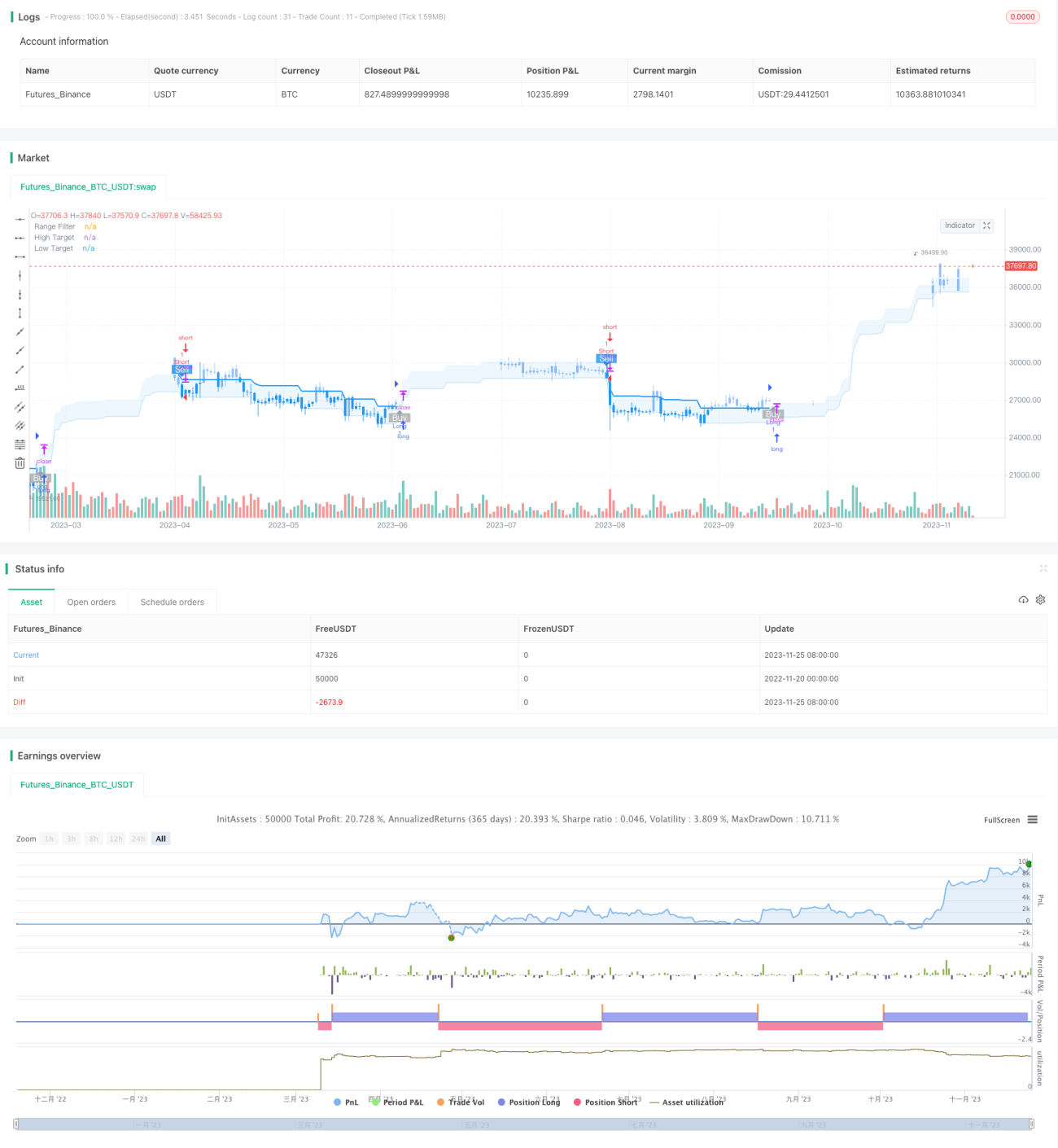
Esta é uma estratégia quantitativa que utiliza julgamento de tendência, filtragem de faixa, confirmação de média móvel dupla e ideias de stop loss. Pode determinar efetivamente a direção da tendência e encontrar um equilíbrio entre maximização de lucro e controle de risco. Através da otimização de parâmetros, aprendizado de máquina e outros meios, a estratégia tem grande espaço para melhoria para alcançar melhores resultados.

/*backtest
start: 2022-11-20 00:00:00
end: 2023-11-26 00:00:00
period: 1d
basePeriod: 1h
exchanges: [{"eid":"Futures_Binance","currency":"BTC_USDT"}]
*/

//@version=5
strategy(title="Range Filter Buy and Sell Strategies", shorttitle="Range Filter Strategies", overlay=true,pyramiding = 5)

// Original Script > @DonovanWall
// Adapted Version > @guikroth
// 
// Updated PineScript to version 5
// Republished by > @tvenn
// Strategizing by > @RonLeigh
//////////////////////////////////////////////////////////////////////////
// Settings for 5min chart, BTCUSDC. For Other coin, change the parameters
//////////////////////////////////////////////////////////////////////////



SS = input.bool(false,"Percentage Take Profit Stop Loss")


longProfitPerc = input.float(title='LongProfit(%)', minval=0.0, step=0.1, defval=1.5) * 0.01

shortProfitPerc = input.float(title='ShortProfit(%)', minval=0.0, step=0.1, defval=1.5) * 0.01


longLossPerc = input.float(title='LongStop(%)', minval=0.0, step=0.1, defval=1.5) * 0.01

shortLossPerc = input.float(title='ShortStop(%)', minval=0.0, step=0.1, defval=1.5) * 0.01


// Color variables
upColor   = color.white
midColor  = #90bff9
downColor = color.blue

// Source
src = input(defval=close, title="Source")

// Sampling Period
// Settings for 5min chart, BTCUSDC. For Other coin, change the paremeters
per = input.int(defval=100, minval=1, title="Sampling Period")

// Range Multiplier
mult = input.float(defval=3.0, minval=0.1, title="Range Multiplier")

// Smooth Average Range
smoothrng(x, t, m) =>
    wper = t * 2 - 1
    avrng = ta.ema(math.abs(x - x[1]), t)
    smoothrng = ta.ema(avrng, wper) * m
    smoothrng
smrng = smoothrng(src, per, mult)

// Range Filter
rngfilt(x, r) =>
    rngfilt = x
    rngfilt := x > nz(rngfilt[1]) ? x - r < nz(rngfilt[1]) ? nz(rngfilt[1]) : x - r : 
       x + r > nz(rngfilt[1]) ? nz(rngfilt[1]) : x + r
    rngfilt
filt = rngfilt(src, smrng)

// Filter Direction
upward = 0.0
upward := filt > filt[1] ? nz(upward[1]) + 1 : filt < filt[1] ? 0 : nz(upward[1])
downward = 0.0
downward := filt < filt[1] ? nz(downward[1]) + 1 : filt > filt[1] ? 0 : nz(downward[1])

// Target Bands
hband = filt + smrng
lband = filt - smrng

// Colors
filtcolor = upward > 0 ? upColor : downward > 0 ? downColor : midColor
barcolor = src > filt and src > src[1] and upward > 0 ? upColor :
   src > filt and src < src[1] and upward > 0 ? upColor : 
   src < filt and src < src[1] and downward > 0 ? downColor : 
   src < filt and src > src[1] and downward > 0 ? downColor : midColor

filtplot = plot(filt, color=filtcolor, linewidth=2, title="Range Filter")

// Target
hbandplot = plot(hband, color=color.new(upColor, 70), title="High Target")
lbandplot = plot(lband, color=color.new(downColor, 70), title="Low Target")

// Fills
fill(hbandplot, filtplot, color=color.new(upColor, 90), title="High Target Range")
fill(lbandplot, filtplot, color=color.new(downColor, 90), title="Low Target Range")

// Bar Color
barcolor(barcolor)

// Break Outs
longCond = bool(na)
shortCond = bool(na)
longCond := src > filt and src > src[1] and upward > 0 or 
   src > filt and src < src[1] and upward > 0
shortCond := src < filt and src < src[1] and downward > 0 or 
   src < filt and src > src[1] and downward > 0

CondIni = 0
CondIni := longCond ? 1 : shortCond ? -1 : CondIni[1]
longCondition = longCond and CondIni[1] == -1
shortCondition = shortCond and CondIni[1] == 1



// alertcondition(longCondition, title="Buy alert on Range Filter", message="Buy alert on Range Filter")
// alertcondition(shortCondition, title="Sell alert on Range Filter", message="Sell alert on Range Filter")
// alertcondition(longCondition or shortCondition, title="Buy and Sell alert on Range Filter", message="Buy and Sell alert on Range Filter")


////////////// 副

sensitivity = input(150, title='Sensitivity')
fastLength = input(20, title='FastEMA Length')
slowLength = input(40, title='SlowEMA Length')
channelLength = input(20, title='BB Channel Length')
multt = input(2.0, title='BB Stdev Multiplier')

DEAD_ZONE = nz(ta.rma(ta.tr(true), 100)) * 3.7

calc_macd(source, fastLength, slowLength) =>
    fastMA = ta.ema(source, fastLength)
    slowMA = ta.ema(source, slowLength)
    fastMA - slowMA

calc_BBUpper(source, length, multt) =>
    basis = ta.sma(source, length)
    dev = multt * ta.stdev(source, length)
    basis + dev

calc_BBLower(source, length, multt) =>
    basis = ta.sma(source, length)
    dev = multt * ta.stdev(source, length)
    basis - dev

t1 = (calc_macd(close, fastLength, slowLength) - calc_macd(close[1], fastLength, slowLength)) * sensitivity

e1 = calc_BBUpper(close, channelLength, multt) - calc_BBLower(close, channelLength, multt)

trendUp = t1 >= 0 ? t1 : 0
trendDown = t1 < 0 ? -1 * t1 : 0

duoad = trendUp > 0 and trendUp > e1

kongad = trendDown > 0 and trendDown > e1



duo =  longCondition and duoad

kong = shortCondition and kongad


//Alerts
plotshape(longCondition  and trendUp > e1 and  trendUp > 0 , title="Buy Signal", text="Buy", textcolor=color.white, style=shape.labelup, size=size.small, location=location.belowbar, color=color.new(#aaaaaa, 20))
plotshape(shortCondition  and trendDown > e1 and  trendDown > 0 , title="Sell Signal", text="Sell", textcolor=color.white, style=shape.labeldown, size=size.small, location=location.abovebar, color=color.new(downColor, 20))




if  longCondition and trendUp > e1 and  trendUp > 0 
    strategy.entry('Long',strategy.long, comment = "buy" )

if  shortCondition and trendDown > e1 and  trendDown > 0 
    strategy.entry('Short',strategy.short, comment = "sell" )




longlimtPrice  = strategy.position_avg_price * (1 + longProfitPerc)
shortlimtPrice = strategy.position_avg_price * (1 - shortProfitPerc)
   
longStopPrice  = strategy.position_avg_price * (1 - longLossPerc)
shortStopPrice = strategy.position_avg_price * (1 + shortLossPerc)



if (strategy.position_size > 0)  and SS == true
    
    strategy.exit(id="Long",comment_profit = "Profit",comment_loss = "StopLoss", stop=longStopPrice,limit = longlimtPrice)
    

if (strategy.position_size < 0)  and SS == true
    
    strategy.exit(id="Short",comment_profit = "Profit",comment_loss = "StopLoss", stop=shortStopPrice,limit = shortlimtPrice)

Mais.