Multi-Timeframe Momentum Breakout Strategie
Überblick
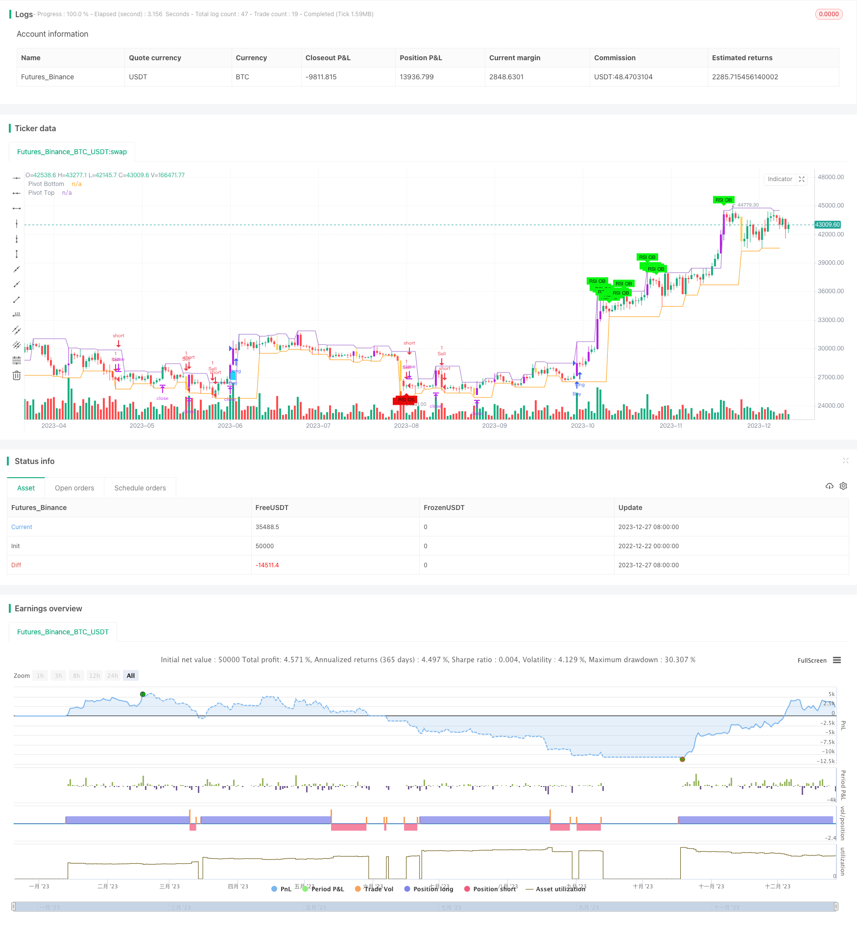
Die Strategie kombiniert mehrere technische Indikatoren wie RSI, ADX, ATR und Dynamik-Indikatoren, um Trend-Beschlüsse und die Erfassung von Durchbruchspunkten zu ermöglichen. Die Strategie kombiniert gleichzeitig die Fibonacci-Rücktrittslinie und die Durchschnittslinie, um die Genauigkeit der Schlüsselpunkte und Trend-Beschlüsse weiter zu verbessern.
Strategieprinzip
Die Richtung und Stärke des Trends wird anhand von Indikatoren wie RSI, ADX, DI+, DI- beurteilt. Der RSI kann Überkauf und Überverkauf widerspiegeln, der ADX die Stärke des Trends und der DI+/DI- den Über- und Überschuss. Die Werte dieser Indikatoren werden in der Tabelle in der oberen rechten Ecke angezeigt, um die Beurteilung zu erleichtern.
Die Kurzzeit-Trend wird durch den 5. und 9. EMA, die Mittelzeit-Trend durch den 21. WMA und die Langzeit-Trend durch den 60. WMA beurteilt. Es handelt sich um ein Mehrkopfsignal, wenn die Mittelzeit-Langzeit-Mittellinie kurzfristig durchbrochen wird.
Die Fibonacci-Rücktrittslinie wird verwendet, um wichtige Unterstützungswerte wie 0,5, 0,618 zu finden. Diese Punkte sind oft potenzielle Wendepunkte.
Setzen Sie einen Stop-Loss-Preis auf Basis der ATR und Stop-Loss-Ratio, um das Risiko zu kontrollieren. Setzen Sie einen Stop-Loss-Preis auf Basis der ATR und Stop-Loss-Ratio, um die Gewinne zu sperren.
Wenn ein RSI-Überkauf-Überverkauf-Signal auftritt, sollten Sie einen Umkehrschluss in Betracht ziehen. Wenn der kurzfristige Durchschnitt überschritten ist (unter) der mittlere und langfristige Durchschnitt und die Handelsmenge größer ist, sollten Sie einen Trend-Eintritt in Betracht ziehen.
Analyse der Stärken
Die Verwendung von mehreren Indikatoren zur Bestimmung der Richtung und Stärke von Trends verbessert die Genauigkeit von Entscheidungen.
Das ATR-basierte Stop-Loss-Stopp-Mechanismus, das die Risiken wirksam kontrolliert.
In Kombination mit Fibonacci-Schlüsselpunkten erhöht sich die Genauigkeit der Umkehrungspunkte.
Die Erhöhung des Handelsvolumens dient als zusätzliche Voraussetzung, um Trends zu verfolgen und falsche Durchbrüche zu vermeiden.
Die Tabelle zeigt die aktuellen Werte von mehreren Indikatoren, um schnelle Entscheidungen zu treffen.
Risikoanalyse
Die Wahrscheinlichkeit, dass ein Indikator ein falsches Signal aussendet, kann nicht vollständig vermieden werden, was zu einem Risiko für Fehlverhalten führt. Die Parameter des Indikators können durch Anpassung der Parameter optimiert werden.
ATR und Stop-Loss-Ratio-Einstellungen beeinflussen den tatsächlichen Stop-Loss-Punkt. Eine zu große oder zu kleine Einstellung des Anteils kann zu einem gewissen Risiko führen und erfordert eine Abwägung.
Die Erhöhung des Handelsvolumens als Einstiegsbedingung kann auch nicht vollständig das Auftreten von Falschbrüchen verhindern, sondern muss in Verbindung mit den Details der Preisentwicklung beurteilt werden.
Der Fibonacci-Punkt ist auch nicht 100% zuverlässig, und der Preis kann direkt über diesen Punkt brechen.
Optimierungsrichtung
Test und Optimierung von Parametern wie RSI, ADX, ATR, um die optimale Kombination zu finden.
Versuchen Sie verschiedene Gleichgewichtskombinationen zu testen, um zu bestimmen, welche die Trendwirkung am besten bestimmen.
Verschiedene Stop-Loss-Stopp-Ratio-Parameter werden getestet, um die Parameter zu ermitteln, die die optimale Risikogewinn-Parameter darstellen.
Die Einbeziehung der BollingerBands-Indikatoren kann in Erwägung gezogen werden, um den Effekt der Erhöhung des Handelsvolumens zu beurteilen.
Zusammenfassen
Die Strategie verwendet eine Vielzahl von Techniken wie Trendbeurteilung, Key-Point-Bewertung, Handelsvolumenanalyse usw. Durch die Optimierung der Parameter werden die Beurteilungsgenauigkeit und die Ertragsfähigkeit weiter verbessert. Die Stop-Loss-Stopp-Einstellung kontrolliert das Risiko und maximiert die Erträge. Die Strategie ist besser geeignet, um mittlere Langstrecken-Trends zu beurteilen und kurzfristige Umkehrwirkungen zu erfassen.
/*backtest
start: 2022-12-22 00:00:00
end: 2023-12-28 00:00:00
period: 1d
basePeriod: 1h
exchanges: [{"eid":"Futures_Binance","currency":"BTC_USDT"}]
*/

// This source code is subject to the terms of the Mozilla Public License 2.0 at https://mozilla.org/MPL/2.0/
// © amit74sharma135

//@version=5

strategy(" KritikSharma Strategy for NIFTY,BNIFTY,NG,CRUDE,WTICrude,BTC,GOLD,SILVER,COPPER", overlay=true)
plotHVB = input.bool(defval=true, title='Plot HVB')
plotPVT = input.bool(defval=false, title='Plot Pivots')
hvbEMAPeriod = input.int(defval=12, minval=1, title='Volume EMA Period')
hvbMultiplier = input.float(defval=1.5, title='Volume Multiplier')
pivotLookup = input.int(defval=2, minval=1, maxval=15, title='Pivot Lookup')
ShowAvg1 = input(false, title="Show trend line", group="TREND LINE Moving Average", tooltip="Display a trend line based on EMA.")
showLines1 = input.bool(defval=false, title="Draw EMA,WMA Line")
ema200_length= input.int(defval=200, minval=1, maxval=500, title='ema1')
ema300_length= input.int(defval=300, minval=1, maxval=500, title='ema2')
wma60_length= input.int(defval=60, minval=1, maxval=100, title='wma60')
ema5 = ta.ema(close, 5)
ema9 = ta.ema(close, 9)
wma21=ta.wma(close,21)
wma60=ta.wma(close,wma60_length)
len1 = input.int(11, minval=1, maxval=500, title="Length", group="TREND LINE Moving Average", tooltip="Set EMA length.")
ema=ta.ema(close, len1)
rsiLength = input.int(14, title="RSI Length", minval=1, maxval=50, group="Table ADX, RSI, DI values with Red, Green, Yellow Signal")
adxLength = input.int(14, title="ADX Length", minval=1, maxval=50, group="Table ADX, RSI, DI values with Red, Green, Yellow Signal")
adxThreshold = input.int(20, title="ADX Threshold", group="Table ADX, RSI, DI values with Red, Green, Yellow Signal")
diThreshold = input.int(25, title="DI Threshold", group="Table ADX, RSI, DI values with Red, Green, Yellow Signal")
atr = input.int(14, title="ATR values", group="Table ADX, RSI, DI values with Red, Green, Yellow Signal")
////////////////////////////////////////////////

hvbBullColor = color.rgb(181, 37, 225)
hvbBearColor = #ffbb00ad

pvtTopColor = color.new(#154bef, 0)
pvtBottomColor = color.new(#b81657, 0)

//////////////////// Pivots ////////////////////
hih = ta.pivothigh(high, pivotLookup, pivotLookup)
lol = ta.pivotlow(low , pivotLookup, pivotLookup)
top1 = ta.valuewhen(hih, high[pivotLookup], 0)
bottom1 = ta.valuewhen(lol, low [pivotLookup], 0)
plot(top1, offset=-pivotLookup, linewidth=1, color=(top1 != top1[1] ? na : (plotPVT ? pvtTopColor : na)), title="Pivot Top")
plot(bottom1, offset=-pivotLookup, linewidth=1, color=(bottom1 != bottom1[1] ? na : (plotPVT ? pvtBottomColor : na)), title="Pivot Bottom")

//////////////////////////////////////Functions
isUp(index) =>
    close[index] > open[index]

isDown(index) =>
    close[index] < open[index]

isObUp(index) =>
    isDown(index + 1) and isUp(index) and close[index] > high[index + 1]

isObDown(index) =>
    isUp(index + 1) and isDown(index) and close[index] < low[index + 1]
////////////////// High Volume Bars //////////////////
volEma = ta.ema(volume, hvbEMAPeriod)
isHighVolume = volume > (hvbMultiplier * volEma)
barcolor(plotHVB and isUp(0) and isHighVolume ? hvbBullColor : na, title="Bullish HVB")
barcolor(plotHVB and isDown(0) and isHighVolume ? hvbBearColor : na, title="Bearish HVB")

// Calculate ADX, DI+,  DI-,RSI,ATR
[diplus, diminus, adx] = ta.dmi(adxLength, adxThreshold)
rsi=ta.rsi(close,rsiLength)
atrValue=ta.atr(atr)

// Check for oversold,Overbought condition
oversold_condition = rsi < 20
overbought_condition = rsi > 80

// Plot Trend Line
trendColor = ema5 > ema9 ? color.rgb(22, 203, 28) : ema5 < ema9 ? color.rgb(224, 15, 15) : na
plot(ShowAvg1? ema:na, color=trendColor, linewidth=6, title="Trend Line Upper Ribbon")

/////////////////////////plot ema,wma
plot(showLines1 ? ta.ema(close, ema200_length) : na, color=color.rgb(102, 110, 103), style=plot.style_line, title="ema1",linewidth = 4)
plot(showLines1 ? ta.ema(close, ema300_length) : na, color=color.rgb(18, 20, 18), style=plot.style_line, title="ema2",linewidth = 4)
plot(showLines1 ? ta.wma(close, wma60_length) : na, color=color.rgb(238, 75, 211), style=plot.style_line, title="wma60",linewidth = 3)

// Plot signals with smaller text
plotshape(oversold_condition ? 1 : na, title="RSI Oversold Signal", color=color.rgb(238, 8, 8), style=shape.labelup, location=location.belowbar, text="RSI OS", textcolor=color.rgb(17, 17, 17), size=size.tiny)
plotshape(overbought_condition ? 1 : na, title="RSI Overbought Signal", color=#08f710, style=shape.labeldown, location=location.abovebar, text="RSI OB", textcolor=color.rgb(8, 8, 8), size=size.tiny)
///////////////////////////////////////////////////////////////////////////////////////////////

// Define input options
showTable = input(false, title="Show Table ADX, RSI, DI values with RED, GREEN and YELLOW Signal")
tablePosition = input.string("Top Right", title="Table Position", options=["Top Right", "Top Left", "Top Center", "Bottom Right", "Bottom Left", "Bottom Center"])

// Define colors for the table cells
colorRsi = rsi > 55 ? color.green : rsi < 45 ? color.red : color.yellow
colorDiPlus = diplus > diThreshold ? color.green : color.red
colorDiMinus = diminus > diThreshold ? color.red : color.green
colorAdx = (rsi < 45 and diplus < diThreshold and diminus > diThreshold and adx > adxThreshold) ? color.red :
           (rsi > 55 and diplus > diThreshold and diminus < diThreshold and adx > adxThreshold) ? color.green :
           color.yellow

// Create the table
var table testTable = na
if showTable
    var position = tablePosition == "Top Right" ? position.top_right :
                   tablePosition == "Top Left" ? position.top_left :
                   tablePosition == "Top Center" ? position.top_center :
                   tablePosition == "Bottom Right" ? position.bottom_right :
                   tablePosition == "Bottom Left" ? position.bottom_left :
                   position.bottom_center

    testTable := table.new(position, columns = 4, rows = 2, border_width = 1, border_color = color.black, frame_width = 1, frame_color = color.black)

    // Column Headings
    table.cell(table_id = testTable, column = 0, row = 0, text = " DI+ ", bgcolor=color.aqua, text_color = color.white)
    table.cell(table_id = testTable, column = 1, row = 0, text = " DI- ", bgcolor=color.aqua, text_color = color.white)
    table.cell(table_id = testTable, column = 2, row = 0, text = " ADX ", bgcolor=color.aqua, text_color = color.white)
    table.cell(table_id = testTable, column = 3, row = 0, text = " RSI ", bgcolor=color.aqua, text_color = color.white)

    // Column values
    table.cell(table_id = testTable, column = 0, row = 1, text = str.tostring(math.round(diplus, 0)), bgcolor=colorDiPlus, text_color = color.black)
    table.cell(table_id = testTable, column = 1, row = 1, text = str.tostring(math.round(diminus, 0)), bgcolor=colorDiMinus, text_color = color.black)
    table.cell(table_id = testTable, column = 2, row = 1, text = str.tostring(math.round(adx, 0)), bgcolor=colorAdx, text_color = color.black)
    table.cell(table_id = testTable, column = 3, row = 1, text = str.tostring(math.round(rsi, 0)), bgcolor=colorRsi, text_color = color.black)


// Initialize variables to keep track of the previous condition
var bool prev_oversold = na
var bool prev_overbought = na

plotshape(ta.crossover(ema,wma60) and isHighVolume,  style=shape.labelup, location=location.belowbar, color=#1adaf3,size=size.small)
plotshape(ta.crossunder(ema,wma60) and isHighVolume,  style=shape.labeldown, location=location.abovebar, color=#f30aa9, size=size.small)
//////////////////////////////////////////////////
plotFibRetracement = input.bool(title="Plot Fibonacci Retracement", defval=false)
fibLevel1 = input.float(title="Fibonacci Level", defval=0.5, minval=0, maxval=1, step=0.01)
fibLevel2 = input.float(title="Fibonacci Level", defval=0.618, minval=0, maxval=1, step=0.01)
fibLevel3 = input.float(title="Fibonacci Level", defval=0.368, minval=0, maxval=1, step=0.01)
// Calculate Fibonacci Levels
highPrice = ta.highest(high, 100)
lowPrice = ta.lowest(low, 100)
priceRange = highPrice - lowPrice
fibonacciLevel1 = lowPrice + priceRange * fibLevel1
fibonacciLevel2 = lowPrice + priceRange * fibLevel2
fibonacciLevel3 = lowPrice + priceRange * fibLevel3

// Plot Fibonacci Levels
if plotFibRetracement
    line.new(x1=bar_index[1], y1=fibonacciLevel1, x2=bar_index, y2=fibonacciLevel1, color=color.blue, width=2)
    line.new(x1=bar_index[1], y1=fibonacciLevel2, x2=bar_index, y2=fibonacciLevel2, color=color.blue, width=2)
    line.new(x1=bar_index[1], y1=fibonacciLevel3, x2=bar_index, y2=fibonacciLevel3, color=color.blue, width=2)
// Draw Trendline
var float trendlineY1 = na
var float trendlineY2 = na

if bar_index % 50 == 0
    trendlineY1 := low
    trendlineY2 := high

// line.new(x1=bar_index, y1=trendlineY1, x2=bar_index - 100, y2=trendlineY2, color=#3708a5, width=2)

////////////////////////////////////////////////entry, exit, profit booking, stoploss///////////////////////
if (rsi > 63 and adx> adxThreshold and diplus>diThreshold)
    strategy.entry("Buy", strategy.long, qty = 1)

if (rsi < 40 and adx> adxThreshold and diminus>diThreshold)
    strategy.entry("Sell", strategy.short, qty = 1)

// Set stop loss and take profit levels
stop_loss = input(1.5, title = "Stop Loss (%)") * atrValue
take_profit = input(4.0, title = "Take Profit (%)") * atrValue
strategy.exit("Take Profit/Stop Loss", from_entry = "Buy", stop = close - stop_loss, limit = close + take_profit)
strategy.exit("Take Profit/Stop Loss", from_entry = "Sell", stop = close + stop_loss, limit = close - take_profit)
////////////////////////