Estrategia de trading de tendencias basada en la divergencia de precios
Descripción general
La estrategia es una estrategia de negociación de tendencias basada en señales de dispersión de precios. Utiliza varios indicadores para detectar señales de dispersión de precios, como RSI, MACD, Stochastics, etc., y se confirma a través de un oscilador de Murray Math.
Principio de estrategia
El núcleo de esta estrategia es la teoría de la dispersión de precios. Cuando el precio es innovador alto pero el indicador no es innovador alto, se llama dispersión de precios de mercado bajista; cuando el precio es innovador bajo pero el indicador no es innovador bajo, se llama dispersión de precios de mercado bajista.
En concreto, las condiciones de ingreso a la estrategia son:
- Detección de señales de dispersión de precios, incluidas dispersiones regulares y dispersiones ocultas
- El oscilador de Murrey Math está dentro de la zona de tendencia correspondiente
Las condiciones de salida son que el oscilador vuelva a la línea media y se iguale.
Análisis de las ventajas
La combinación de la teoría de la dispersión de precios y la confirmación de tendencias tiene las siguientes ventajas:
- El uso de señales dispersas de precios para detectar posibles cambios de tendencia
- Los osciladores de aplicaciones confirman la tendencia actual y evitan falsas rupturas
- Combinaciones de indicadores y parámetros que se pueden ajustar con flexibilidad
- Seguir las tendencias y evitar pérdidas
- Las reglas de lógica son claras y hay mucho espacio para optimizar el código.
Análisis de riesgos
Los principales riesgos son los siguientes:
- Las señales de dispersión de precios pueden ser falsas y no se puede confirmar una reversión de tendencia.
- La configuración incorrecta de los parámetros del oscilador puede causar una fuga de entrada y una oportunidad de negociación perdida
- El exceso de inclinación de las posiciones exentas conlleva un mayor riesgo de pérdidas
- El número de transacciones y los costos de los puntos de deslizamiento pueden aumentar durante las fluctuaciones extremas
Se recomienda establecer paros, ajustar posiciones y optimizar la combinación de parámetros para reducir el riesgo.
Dirección de optimización
La estrategia tiene espacio para ser optimizada aún más:
- Agrega algoritmos de aprendizaje automático para optimizar el conjunto de parámetros en tiempo real
- Aumentar las técnicas de parada de pérdidas adaptativas, como el seguimiento de la parada, la parada promedio, etc.
- Mejora de la relación de ruido de la señal, combinada con más indicadores y condiciones de filtración
- Ajuste dinámico de los parámetros del oscilador para optimizar el juicio de tendencias
- Optimización de la gestión de riesgos, establecimiento de límites de retiro máximo, etc.
Resumir
La estrategia integra la teoría de la dispersión de precios y los indicadores de análisis de tendencias para detectar con eficacia los posibles puntos de cambio de tendencia. La combinación de medidas de gestión de riesgos optimizadas puede obtener una mejor tasa de rendimiento de la estrategia. En el futuro, se puede optimizar con métodos avanzados como el aprendizaje automático para obtener ganancias extras más estables.
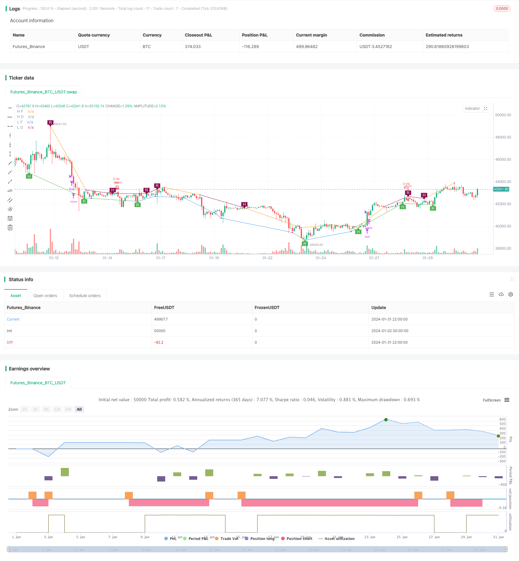
/*backtest
start: 2024-01-02 00:00:00
end: 2024-02-01 00:00:00
period: 2h
basePeriod: 15m
exchanges: [{"eid":"Futures_Binance","currency":"BTC_USDT"}]
*/

//@version=2
//
// Title:   [STRATEGY][UL]Price Divergence Strategy V1
// Author:  JustUncleL
// Date:    23-Oct-2016
// Version: v1.0
//
// Description:
//  A trend trading strategy the uses Price Divergence detection signals, that
//  are confirmed by the "Murrey's Math Oscillator" (Donchanin Channel based).
//
//  *** USE AT YOUR OWN RISK ***
//
// Mofidifications:
//  1.0 - original
//
// References:
//  Strategy Based on:
//  - [RS]Price Divergence Detector V2 by RicardoSantos
//  - UCS_Murrey's Math Oscillator by Ucsgears
//  Some Code borrowed from:
//  - "Strategy Code Example by JayRogers"
//  Information on Divergence Trading:
//  - http://www.babypips.com/school/high-school/trading-divergences
//
strategy(title='[STRATEGY][UL]Price Divergence Strategy v1.0', pyramiding=0, overlay=true, initial_capital=10000, calc_on_every_tick=false,
         currency=currency.USD,default_qty_type=strategy.percent_of_equity,default_qty_value=10)
//  ||  General Input:
method = input(title='Method (0=rsi, 1=macd, 2=stoch, 3=volume, 4=acc/dist, 5=fisher, 6=cci):',  defval=1, minval=0, maxval=6)
SHOW_LABEL = input(title='Show Labels', type=bool, defval=true)
SHOW_CHANNEL = input(title='Show Channel', type=bool, defval=false)
uHid = input(true,title="Use Hidden Divergence in Strategy")
uReg = input(true,title="Use Regular Divergence in Strategy")
//  ||  RSI / STOCH / VOLUME / ACC/DIST Input:
rsi_smooth = input(title='RSI/STOCH/Volume/ACC-DIST/Fisher/cci Smooth:',  defval=5)
//  ||  MACD Input:
macd_src = input(title='MACD Source:', defval=close)
macd_fast = input(title='MACD Fast:',  defval=12)
macd_slow = input(title='MACD Slow:',  defval=26)
macd_smooth = input(title='MACD Smooth Signal:',  defval=9)
//  ||  Functions:
f_top_fractal(_src)=>_src[4] < _src[2] and _src[3] < _src[2] and _src[2] > _src[1] and _src[2] > _src[0]
f_bot_fractal(_src)=>_src[4] > _src[2] and _src[3] > _src[2] and _src[2] < _src[1] and _src[2] < _src[0]
f_fractalize(_src)=>f_top_fractal(_src) ? 1 : f_bot_fractal(_src) ? -1 : 0

//  ||••>   START MACD FUNCTION
f_macd(_src, _fast, _slow, _smooth)=>
    _fast_ma = sma(_src, _fast)
    _slow_ma = sma(_src, _slow)
    _macd = _fast_ma-_slow_ma
    _signal = ema(_macd, _smooth)
    _hist = _macd - _signal
//  ||<••   END MACD FUNCTION

//  ||••>   START ACC/DIST FUNCTION
f_accdist(_smooth)=>_return=sma(cum(close==high and close==low or high==low ? 0 : ((2*close-low-high)/(high-low))*volume), _smooth)
//  ||<••   END ACC/DIST FUNCTION

//  ||••>   START FISHER FUNCTION
f_fisher(_src, _window)=>
    _h = highest(_src, _window)
    _l = lowest(_src, _window)
    _value0 = .66 * ((_src - _l) / max(_h - _l, .001) - .5) + .67 * nz(_value0[1])
    _value1 = _value0 > .99 ? .999 : _value0 < -.99 ? -.999 : _value0
    _fisher = .5 * log((1 + _value1) / max(1 - _value1, .001)) + .5 * nz(_fisher[1])
//  ||<••   END FISHER FUNCTION

method_high = method == 0 ? rsi(high, rsi_smooth) :
  method == 1 ? f_macd(macd_src, macd_fast, macd_slow, macd_smooth) :
  method == 2 ? stoch(close, high, low, rsi_smooth) :
  method == 3 ? sma(volume, rsi_smooth) :
  method == 4 ? f_accdist(rsi_smooth) :
  method == 5 ? f_fisher(high, rsi_smooth) :
  method == 6 ? cci(high, rsi_smooth) :
  na

method_low = method == 0 ? rsi(low, rsi_smooth) :
  method == 1 ? f_macd(macd_src, macd_fast, macd_slow, macd_smooth) :
  method == 2 ? stoch(close, high, low, rsi_smooth) :
  method == 3 ? sma(volume, rsi_smooth) :
  method == 4 ? f_accdist(rsi_smooth) :
  method == 5 ? f_fisher(low, rsi_smooth) :
  method == 6 ? cci(low, rsi_smooth) :
  na

fractal_top = f_fractalize(method_high) > 0 ? method_high[2] : na
fractal_bot = f_fractalize(method_low) < 0 ? method_low[2] : na

high_prev = valuewhen(fractal_top, method_high[2], 1)
high_price = valuewhen(fractal_top, high[2], 1)
low_prev = valuewhen(fractal_bot, method_low[2], 1)
low_price = valuewhen(fractal_bot, low[2], 1)

regular_bearish_div = fractal_top and high[2] > high_price and method_high[2] < high_prev
hidden_bearish_div = fractal_top and high[2] < high_price and method_high[2] > high_prev
regular_bullish_div = fractal_bot and low[2] < low_price and method_low[2] > low_prev
hidden_bullish_div = fractal_bot and low[2] > low_price and method_low[2] < low_prev

plot(title='H F', series=fractal_top ? high[2] : na, color=regular_bearish_div or hidden_bearish_div ? maroon : not SHOW_CHANNEL ? na : silver, offset=-2)
plot(title='L F', series=fractal_bot ? low[2] : na, color=regular_bullish_div or hidden_bullish_div ? green : not SHOW_CHANNEL ? na : silver, offset=-2)
plot(title='H D', series=fractal_top ? high[2] : na, style=circles, color=regular_bearish_div or hidden_bearish_div ? maroon : not SHOW_CHANNEL ? na : silver, linewidth=3, offset=-2)
plot(title='L D', series=fractal_bot ? low[2] : na, style=circles, color=regular_bullish_div or hidden_bullish_div ? green : not SHOW_CHANNEL ? na : silver, linewidth=3, offset=-2)

plotshape(title='+RBD', series=not SHOW_LABEL ? na : regular_bearish_div ? high[2] : na, text='R', style=shape.labeldown, location=location.absolute, color=maroon, textcolor=white, offset=-2)
plotshape(title='+HBD', series=not SHOW_LABEL ? na : hidden_bearish_div ? high[2] : na, text='H', style=shape.labeldown, location=location.absolute, color=maroon, textcolor=white, offset=-2)
plotshape(title='-RBD', series=not SHOW_LABEL ? na : regular_bullish_div ? low[2] : na, text='R', style=shape.labelup, location=location.absolute, color=green, textcolor=white, offset=-2)
plotshape(title='-HBD', series=not SHOW_LABEL ? na : hidden_bullish_div ? low[2] : na, text='H', style=shape.labelup, location=location.absolute, color=green, textcolor=white, offset=-2)

// Code borrowed from UCS_Murrey's Math Oscillator by Ucsgears
//  - UCS_MMLO
// Inputs
length = input(100, minval = 10, title = "MMLO Look back Length")
quad   = input(2, minval = 1, maxval = 4, step = 1, title = "Mininum Quadrant for MMLO Support")
mult = 0.125

// Donchanin Channel
hi = highest(high, length)
lo = lowest(low, length)
range = hi - lo
multiplier = (range) * mult
midline = lo + multiplier * 4

oscillator = (close - midline)/(range/2)

a = oscillator > 0
b = oscillator > 0 and oscillator > mult*2
c = oscillator > 0 and oscillator > mult*4
d = oscillator > 0 and oscillator > mult*6

z = oscillator < 0
y = oscillator < 0 and oscillator < -mult*2
x = oscillator < 0 and oscillator < -mult*4
w = oscillator < 0 and oscillator < -mult*6


//  Strategy: (Thanks to JayRogers)
// === STRATEGY RELATED INPUTS ===
//tradeInvert     = input(defval = false, title = "Invert Trade Direction?")
// the risk management inputs
inpTakeProfit   = input(defval = 0, title = "Take Profit Points", minval = 0)
inpStopLoss     = input(defval = 0, title = "Stop Loss Points", minval = 0)
inpTrailStop    = input(defval = 100, title = "Trailing Stop Loss Points", minval = 0)
inpTrailOffset  = input(defval = 0, title = "Trailing Stop Loss Offset Points", minval = 0)

// === RISK MANAGEMENT VALUE PREP ===
// if an input is less than 1, assuming not wanted so we assign 'na' value to disable it.
useTakeProfit   = inpTakeProfit  >= 1 ? inpTakeProfit  : na
useStopLoss     = inpStopLoss    >= 1 ? inpStopLoss    : na
useTrailStop    = inpTrailStop   >= 1 ? inpTrailStop   : na
useTrailOffset  = inpTrailOffset >= 1 ? inpTrailOffset : na

// === STRATEGY - LONG POSITION EXECUTION ===
enterLong() => ((uReg and regular_bullish_div) or (uHid and hidden_bullish_div)) and (quad==1? a[1]: quad==2?b[1]: quad==3?c[1]: quad==4?d[1]: false)// functions can be used to wrap up and work out complex conditions
exitLong() => oscillator <= 0
strategy.entry(id = "Buy", long = true, when = enterLong() )// use function or simple condition to decide when to get in
strategy.close(id = "Buy", when = exitLong() )// ...and when to get out

// === STRATEGY - SHORT POSITION EXECUTION ===
enterShort() => ((uReg and regular_bearish_div) or (uHid and hidden_bearish_div)) and (quad==1? z[1]: quad==2?y[1]: quad==3?x[1]: quad==4?w[1]: false)
exitShort() => oscillator >= 0
strategy.entry(id = "Sell", long = false, when = enterShort())
strategy.close(id = "Sell", when = exitShort() )

// === STRATEGY RISK MANAGEMENT EXECUTION ===
// finally, make use of all the earlier values we got prepped
strategy.exit("Exit Buy", from_entry = "Buy", profit = useTakeProfit, loss = useStopLoss, trail_points = useTrailStop, trail_offset = useTrailOffset)
strategy.exit("Exit Sell", from_entry = "Sell", profit = useTakeProfit, loss = useStopLoss, trail_points = useTrailStop, trail_offset = useTrailOffset)


//EOF