Stratégie de suivi de tendance basée sur kNN


Date de création: 2023-12-08 11:33:31 Dernière modification: 2023-12-08 11:33:31
Copier: 0 Nombre de clics: 1511
1
Suivre
1621
Abonnés

Stratégie de suivi de tendance basée sur kNN

Aperçu

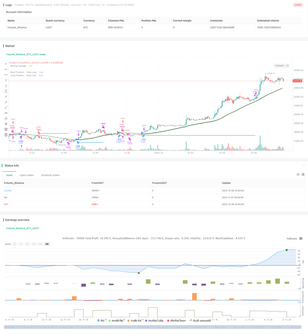
Cette stratégie utilise des algorithmes d’apprentissage de la machine à proximité de k pour prédire les tendances du marché et générer des signaux de position longue et de position vide en fonction des résultats de la prévision. La stratégie prend en compte des facteurs tels que les données historiques, les indicateurs techniques, les caractéristiques du marché grâce à la formation de la dynamique du modèle de kNN et permet l’automatisation des transactions de suivi des tendances.

Principe de stratégie

  1. La collecte de données d’entraînement: collecte des séquences chronologiques telles que le cours de clôture historique, le volume des transactions, ainsi que des indicateurs techniques tels que le RSI, le CCI.

  2. Pré-traitement des données: homogénéisation des valeurs de l’indicateur dans la plage 0 à 100.

  3. Entraînement du modèle kNN: saisissez deux caractéristiques du modèle kNN actuel, calculez la distance en euros entre ces vecteurs caractéristiques et les vecteurs caractéristiques historiques, sélectionnez la distance la plus proche de k échantillons historiques, et statistiquez la répartition des étiquettes ((multi-têtes ou tête vide) de ces k échantillons.

  4. Obtenir une prévision: prédire la tendance actuelle du marché en fonction des balises de k échantillons les plus proches. Si la prévision est à plusieurs têtes, produire un signal de position longue; si la prévision est à vide, produire un signal de position vide.

  5. Les filtres de stop loss, de contrôle de position et d’une moyenne mobile sont utilisés pour effectuer des transactions.

Avantages stratégiques

  1. L’algorithme d’apprentissage automatique est utilisé pour identifier automatiquement la forme de la technologie, sans intervention humaine.

  2. La flexibilité de choisir différents indicateurs techniques comme caractéristiques du modèle et des stratégies d’optimisation en temps réel.

  3. Un mécanisme rigoureux de contrôle des risques, comme l’intégration de stop-loss et la gestion des positions.

  4. La visualisation présente une ligne de rupture claire et intuitive.

Les risques et les solutions

  1. Les prédictions d’apprentissage automatique peuvent être fausses. Des modèles d’optimisation tels que des valeurs de k, des vecteurs de caractéristiques et des intervalles de temps d’échantillonnage peuvent être choisis.

  2. Les transactions unilatérales présentent un risque potentiel. Des transactions bilatérales peuvent être ajoutées au code pour supprimer les bugs.

  3. Une mauvaise configuration des paramètres peut entraîner des transactions excessives. Les paramètres tels que la taille de la position, la fréquence des transactions doivent être ajustés de manière appropriée.

Direction d’optimisation

  1. Tester différents types d’indicateurs techniques comme caractéristiques d’entrée de kNN.

  2. Essayez d’autres méthodes de mesure de la distance, comme la distance de Manhattan.

  3. Ajustez la taille de la position à l’aide de la distance d’échantillonnage ou de la classification de la qualité.

  4. Ajouter des ensembles d’entraînement de modèles, des ensembles de test et des divisions pour optimiser le défilement.

Résumer

Cette stratégie utilise l’algorithme classique kNN pour prédire les tendances du marché et suivre les tendances en fonction des signaux de prévision. La stratégie est paramétrable et contrôlable en termes de risques, ce qui permet aux utilisateurs d’obtenir un programme de trading automatisé efficace. Les utilisateurs peuvent améliorer continuellement la performance de la stratégie en ajustant la combinaison d’indicateurs techniques, en optimisant les modèles de surparamètres, etc.

Code source de la stratégie
/*backtest
start: 2023-11-07 00:00:00
end: 2023-12-07 00:00:00
period: 1h
basePeriod: 15m
exchanges: [{"eid":"Futures_Binance","currency":"BTC_USDT"}]
*/

// This source code is subject to the terms of the Mozilla Public License 2.0 at https://mozilla.org/MPL/2.0/
// © sosacur01

//@version=5
strategy(title=" kNN-based| Trend Following  | Trend Following", overlay=true, pyramiding=1, commission_type=strategy.commission.percent, commission_value=0.2, initial_capital=10000)

//==========================================
// This script, based on Capissimo's original indicator code, transforms a kNN-based machine learning indicator into a TradingView strategy.
// It incorporates a backtest date range filter, on/off controls for long and short positions, a moving average filter, and dynamic risk management for adaptive position sizing.
// Credit to Capissimo for the foundational kNN algorithm.
//==========================================

//BACKTEST RANGE
useDateFilter = input.bool(true, title="Filter Date Range of Backtest",
     group="Backtest Time Period")
backtestStartDate = input(timestamp("1 jan 2017"), 
     title="Start Date", group="Backtest Time Period",
     tooltip="This start date is in the time zone of the exchange " + 
     "where the chart's instrument trades. It doesn't use the time " + 
     "zone of the chart or of your computer.")
backtestEndDate = input(timestamp("1 Jul 2100"),
     title="End Date", group="Backtest Time Period",
     tooltip="This end date is in the time zone of the exchange " + 
     "where the chart's instrument trades. It doesn't use the time " + 
     "zone of the chart or of your computer.")
inTradeWindow = true
if not inTradeWindow and inTradeWindow[1]
    strategy.cancel_all()
    strategy.close_all(comment="Date Range Exit")

//--------------------------------------

//LONG/SHORT POSITION ON/OFF INPUT
LongPositions   = input.bool(title='On/Off Long Postion', defval=true, group="Long & Short Position")
ShortPositions  = input.bool(title='On/Off Short Postion', defval=true, group="Long & Short Position")

//--------------------------------------
// kNN-based Strategy (FX and Crypto)
// Description: 
// This strategy uses a classic machine learning algorithm - k Nearest Neighbours (kNN) - 
// to let you find a prediction for the next (tomorrow's, next month's, etc.) market move. 
// Being an unsupervised machine learning algorithm, kNN is one of the most simple learning algorithms. 

// To do a prediction of the next market move, the kNN algorithm uses the historic data, 
// collected in 3 arrays - feature1, feature2 and directions, - and finds the k-nearest 
// neighbours of the current indicator(s) values. 

// The two dimensional kNN algorithm just has a look on what has happened in the past when 
// the two indicators had a similar level. It then looks at the k nearest neighbours, 
// sees their state and thus classifies the current point.

// The kNN algorithm offers a framework to test all kinds of indicators easily to see if they 
// have got any *predictive value*. One can easily add cog, wpr and others.
// Note: TradingViews's playback feature helps to see this strategy in action.
// Warning: Signals ARE repainting.

// Style tags: Trend Following, Trend Analysis
// Asset class: Equities, Futures, ETFs, Currencies and Commodities
// Dataset: FX Minutes/Hours+++/Days

//-- Preset Dates

int startdate = timestamp('01 Jan 2000 00:00:00 GMT+10')
int stopdate  = timestamp('31 Dec 2025 23:45:00 GMT+10')

//-- Inputs

StartDate  = input  (startdate, 'Start Date', group="kNN-based Inputs")
StopDate   = input  (stopdate,  'Stop Date', group="kNN-based Inputs")
Indicator  = input.string('RSI',     'Indicator',   ['RSI','ROC','CCI','Volume','All'], group="kNN-based Inputs")
ShortWinow = input.int   (8,        'Short Period [1..n]', 1, group="kNN-based Inputs")
LongWindow = input.int   (29,        'Long Period [2..n]',  2, group="kNN-based Inputs")
BaseK      = input.int   (400,       'Base No. of Neighbours (K) [5..n]', 5, group="kNN-based Inputs")
Filter     = input.bool  (false,     'Volatility Filter', group="kNN-based Inputs")
Bars       = input.int   (300,       'Bar Threshold [2..5000]', 2, 5000, group="kNN-based Inputs")

//-- Constants

var int BUY   = 1
var int SELL  =-1
var int CLEAR = 0

var int k     = math.floor(math.sqrt(BaseK))  // k Value for kNN algo

//-- Variable

// Training data, normalized to the range of [0,...,100]
var array<float> feature1   = array.new_float(0)  // [0,...,100]
var array<float> feature2   = array.new_float(0)  //    ...
var array<int>   directions = array.new_int(0)    // [-1; +1]

// Result data
var array<int>   predictions = array.new_int(0)
var float        prediction  = 0.0
var array<int>   bars        = array.new<int>(1, 0) // array used as a container for inter-bar variables

// Signals
var int          signal      = CLEAR

//-- Functions

minimax(float x, int p, float min, float max) => 
    float hi = ta.highest(x, p), float lo = ta.lowest(x, p)
    (max - min) * (x - lo)/(hi - lo) + min

cAqua(int g) => g>9?#0080FFff:g>8?#0080FFe5:g>7?#0080FFcc:g>6?#0080FFb2:g>5?#0080FF99:g>4?#0080FF7f:g>3?#0080FF66:g>2?#0080FF4c:g>1?#0080FF33:#00C0FF19
cPink(int g) => g>9?#FF0080ff:g>8?#FF0080e5:g>7?#FF0080cc:g>6?#FF0080b2:g>5?#FF008099:g>4?#FF00807f:g>3?#FF008066:g>2?#FF00804c:g>1?#FF008033:#FF008019

inside_window(float start, float stop) =>  
    time >= start and time <= stop ? true : false

//-- Logic

bool window = true

// 3 pairs of predictor indicators, long and short each
float rs = ta.rsi(close,   LongWindow),        float rf = ta.rsi(close,   ShortWinow)
float cs = ta.cci(close,   LongWindow),        float cf = ta.cci(close,   ShortWinow)
float os = ta.roc(close,   LongWindow),        float of = ta.roc(close,   ShortWinow)
float vs = minimax(volume, LongWindow, 0, 99), float vf = minimax(volume, ShortWinow, 0, 99)

// TOADD or TOTRYOUT:
//    ta.cmo(close, LongWindow), ta.cmo(close, ShortWinow)
//    ta.mfi(close, LongWindow), ta.mfi(close, ShortWinow)
//    ta.mom(close, LongWindow), ta.mom(close, ShortWinow)

float f1 = switch Indicator
    'RSI'    => rs 
    'CCI'    => cs 
    'ROC'    => os 
    'Volume' => vs 
    => math.avg(rs, cs, os, vs)

float f2 = switch Indicator
    'RSI'    => rf 
    'CCI'    => cf
    'ROC'    => of
    'Volume' => vf 
    => math.avg(rf, cf, of, vf)

// Classification data, what happens on the next bar
int class_label = int(math.sign(close[1] - close[0])) // eq. close[1]<close[0] ? SELL: close[1]>close[0] ? BUY : CLEAR

// Use particular training period
if window
    // Store everything in arrays. Features represent a square 100 x 100 matrix,
    // whose row-colum intersections represent class labels, showing historic directions
    array.push(feature1, f1)
    array.push(feature2, f2)
    array.push(directions, class_label)

// Ucomment the followng statement (if barstate.islast) and tab everything below
// between BOBlock and EOBlock marks to see just the recent several signals gradually 
// showing up, rather than all the preceding signals

//if barstate.islast   

//==BOBlock	

// Core logic of the algorithm
int   size    = array.size(directions)
float maxdist = -999.0
// Loop through the training arrays, getting distances and corresponding directions.
for i=0 to size-1
    // Calculate the euclidean distance of current point to all historic points,
    // here the metric used might as well be a manhattan distance or any other.
    float d = math.sqrt(math.pow(f1 - array.get(feature1, i), 2) + math.pow(f2 - array.get(feature2, i), 2))
    
    if d > maxdist
        maxdist := d
        if array.size(predictions) >= k
            array.shift(predictions)
        array.push(predictions, array.get(directions, i))
        
//==EOBlock	

// Note: in this setup there's no need for distances array (i.e. array.push(distances, d)),
//       but the drawback is that a sudden max value may shadow all the subsequent values.
// One of the ways to bypass this is to:
// 1) store d in distances array,
// 2) calculate newdirs = bubbleSort(distances, directions), and then 
// 3) take a slice with array.slice(newdirs) from the end
    	
// Get the overall prediction of k nearest neighbours
prediction := array.sum(predictions)   

bool filter = Filter ? ta.atr(10) > ta.atr(40) : true // filter out by volatility or ex. ta.atr(1) > ta.atr(10)...

// Now that we got a prediction for the next market move, we need to make use of this prediction and 
// trade it. The returns then will show if everything works as predicted.
// Over here is a simple long/short interpretation of the prediction, 
// but of course one could also use the quality of the prediction (+5 or +1) in some sort of way,
// ex. for position sizing.

bool long  = prediction > 0 and filter
bool short = prediction < 0 and filter
bool clear = not(long and short)

if array.get(bars, 0)==Bars    // stop by trade duration
    signal := CLEAR
    array.set(bars, 0, 0)
else
    array.set(bars, 0, array.get(bars, 0) + 1)

signal := long ? BUY : short ? SELL : clear ? CLEAR : nz(signal[1])

int  changed         = ta.change(signal)
bool startLongTrade  = changed and signal==BUY 
bool startShortTrade = changed and signal==SELL 
// bool endLongTrade    = changed and signal==SELL
// bool endShortTrade   = changed and signal==BUY  
bool clear_condition = changed and signal==CLEAR //or (changed and signal==SELL) or (changed and signal==BUY)

float maxpos = ta.highest(high, 10)
float minpos = ta.lowest (low,  10)


//----//MA INPUTS
MAFilter        = input.bool(title='Use MA as Filter', defval=true, group = "MA Inputs")
averageType1    = input.string(defval="SMA", group="MA Inputs", title="MA Type", options=["SMA", "EMA", "WMA", "HMA", "RMA", "SWMA", "ALMA", "VWMA", "VWAP"])
averageLength1  = input.int(defval=40, title="MA Length", group="MA Inputs")
averageSource1  = input(close, title="MA Source", group="MA Inputs")        

//MA TYPE
MovAvgType1(averageType1, averageSource1, averageLength1) =>
	switch str.upper(averageType1)
        "SMA"  => ta.sma(averageSource1, averageLength1)
        "EMA"  => ta.ema(averageSource1, averageLength1)
        "WMA"  => ta.wma(averageSource1, averageLength1)
        "HMA"  => ta.hma(averageSource1, averageLength1)
        "RMA"  => ta.rma(averageSource1, averageLength1)
        "SWMA" => ta.swma(averageSource1)
        "ALMA" => ta.alma(averageSource1, averageLength1, 0.85, 6)
        "VWMA" => ta.vwma(averageSource1, averageLength1)
        "VWAP" => ta.vwap(averageSource1)
        => runtime.error("Moving average type '" + averageType1 + 
             "' not found!"), na


// MA COLOR VALUES
ma = MovAvgType1(averageType1, averageSource1, averageLength1)
ma_plot = close > ma ? color.rgb(54, 111, 56) : color.rgb(54, 111, 56, 52)

// MA BUY/SELL CONDITIONS
bullish_ma = MAFilter ? close > ma  : inTradeWindow
bearish_ma = MAFilter ? close < ma  : inTradeWindow

// MA ALTERNATING PLOT
plot(MAFilter ? ma : na, color=ma_plot, title="Moving Average", linewidth=3)
//--------------------------------------

//ENTRIES AND EXITS
long_entry  = if inTradeWindow and startLongTrade and bullish_ma and LongPositions
    true
long_exit   = if inTradeWindow and startShortTrade
    true

short_entry = if inTradeWindow and startShortTrade and bearish_ma and ShortPositions
    true
short_exit  = if inTradeWindow and startLongTrade
    true
    
//--------------------------------------
//RISK MANAGEMENT - SL, MONEY AT RISK, POSITION SIZING
atrPeriod                = input.int(7, "ATR Length", group="Risk Management Inputs")
sl_atr_multiplier        = input.float(title="Long Position - Stop Loss - ATR Multiplier", defval=2, group="Risk Management Inputs", step=0.5)
sl_atr_multiplier_short  = input.float(title="Short Position - Stop Loss - ATR Multiplier", defval=2, group="Risk Management Inputs", step=0.5)
i_pctStop                = input.float(2, title="% of Equity at Risk", step=.5, group="Risk Management Inputs")/100

//ATR VALUE
_atr = ta.atr(atrPeriod)

//CALCULATE LAST ENTRY PRICE
lastEntryPrice = strategy.opentrades.entry_price(strategy.opentrades - 1)

//STOP LOSS - LONG POSITIONS 
var float sl = na

//CALCULTE SL WITH ATR AT ENTRY PRICE - LONG POSITION
if (strategy.position_size[1] != strategy.position_size)
    sl := lastEntryPrice - (_atr * sl_atr_multiplier)

//IN TRADE - LONG POSITIONS
inTrade = strategy.position_size > 0

//PLOT SL - LONG POSITIONS
plot(inTrade ? sl : na, color=color.blue, style=plot.style_circles, title="Long Position - Stop Loss")

//CALCULATE ORDER SIZE - LONG POSITIONS
positionSize = (strategy.equity * i_pctStop) / (_atr * sl_atr_multiplier)

//============================================================================================

//STOP LOSS - SHORT POSITIONS 
var float sl_short = na

//CALCULTE SL WITH ATR AT ENTRY PRICE - SHORT POSITIONS 
if (strategy.position_size[1] != strategy.position_size)
    sl_short := lastEntryPrice + (_atr * sl_atr_multiplier_short)

//IN TRADE SHORT POSITIONS
inTrade_short = strategy.position_size < 0

//PLOT SL - SHORT POSITIONS
plot(inTrade_short ? sl_short : na, color=color.red, style=plot.style_circles, title="Short Position - Stop Loss")

//CALCULATE ORDER - SHORT POSITIONS
positionSize_short = (strategy.equity * i_pctStop) / (_atr * sl_atr_multiplier_short) 


//===============================================

//LONG STRATEGY
strategy.entry("Long", strategy.long, comment="Long", when = long_entry and not short_entry, qty=positionSize)
if (strategy.position_size > 0)
    strategy.close("Long", when = (long_exit), comment="Close Long")
    strategy.exit("Long", stop = sl, comment="Exit Long")

//SHORT STRATEGY
strategy.entry("Short", strategy.short, comment="Short", when = short_entry and not long_entry, qty=positionSize_short)
if (strategy.position_size < 0) 
    strategy.close("Short", when = (short_exit), comment="Close Short")
    strategy.exit("Short", stop = sl_short, comment="Exit Short")

//ONE DIRECTION TRADING COMMAND (BELLOW ONLY ACTIVATE TO CORRECT BUGS)
//strategy.risk.allow_entry_in(strategy.direction.long)