kNN 기반 트렌드 추종 전략


생성 날짜: 2023-12-08 11:33:31 마지막으로 수정됨: 2023-12-08 11:33:31
복사: 0 클릭수: 1511
avatar of ChaoZhang ChaoZhang
1
집중하다
1621
수행원

kNN 기반 트렌드 추종 전략

개요

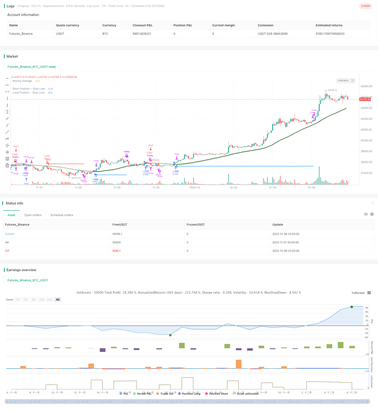
이 전략은 k 근접 (kNN) 기계 학습 알고리즘을 사용하여 시장 추세를 예측하고, 예측 결과에 따라 긴 포지션과 빈 포지션 신호를 생성한다. 이 전략은 종합적으로 역사적 데이터, 기술 지표와 같은 여러 요소를 고려하고, kNN 모델 동력을 통해 시장 특성을 획득하고, 자동화 된 트렌드 추적 거래를 구현한다.

전략 원칙

  1. 훈련 데이터를 수집합니다. 역사적인 종식 가격, 거래량과 같은 시간 순서, RSI, CCI와 같은 기술 지표들을 수집합니다.

  2. 데이터 전처리: 지표값을 0-100의 범위로 정형화한다.

  3. 트레이닝 kNN 모델: 현재 kNN 모델의 두 가지 특징을 입력하고, 이들 특징 벡터와 역사 특징 벡터 사이의 유럽식 거리를 계산하고, 가장 가까운 k개의 역사 샘플의 거리를 선택하고, 이 k개의 샘플의 레이블 ((多頭 or 空頭) 분포 상황을 통계한다.

  4. 예측을 얻는다: k의 가장 가까운 이웃 샘플의 표기에 따라 현재 시장의 움직임을 예측한다. 예측이 다목적이라면, 긴 포지션 신호를 생성한다. 예측이 공백이라면, 빈 포지션 신호를 생성한다.

  5. 스톱로스, 포지션 제어, 이동 평균 등의 필터와 함께 거래한다.

전략적 이점

  1. 기계 학습 알고리즘을 사용하여 기술 형태를 자동으로 식별하고, 사람의 개입이 필요하지 않습니다.

  2. 다양한 기술 지표를 모델 특성으로 선택하여 실시간 최적화 전략을 적용할 수 있습니다.

  3. 통합된 스톱로스, 포지션 관리 등과 같은 엄격한 위험 제어 장치

  4. 시각화 상쇄선, 명확한 직관.

위험과 해결책

  1. 기계학습 예측에는 오류가 발생할 수 있다. 적절한 k값, 특징 벡터, 샘플링 시간 범위 등의 최적화 모델을 선택할 수 있다.

  2. 일방적인 거래는 잠재적인 위험이다. 코드에서 쌍방적인 거래를 추가하면 버그를 제거할 수 있다.

  3. 매개 변수 설정이 잘못되면 과도한 거래가 발생할 수 있다. 포지션 크기, 거래 빈도 등의 매개 변수들을 적절히 조정해야 한다.

최적화 방향

  1. 다양한 유형의 기술 지표를 kNN 입력 특성으로 테스트한다.

  2. 맨해튼 거리처럼 다른 거리 측정 방법을 시도해 보세요.

  3. 샘플 거리 또는 분류 질량을 사용하여 포지션 크기를 조정하십시오.

  4. 모델 트레이닝 세트를 추가하고, 테스트 세트를 분할하여, 스크롤 최적화를 구현한다.

요약하다

이 전략은 고전적인 kNN 알고리즘을 사용하여 시장 추세를 예측하고 예측 신호에 따라 추세를 따라 거래한다. 이 전략은 매개 변수를 조정할 수 있고, 위험을 제어할 수 있는 특징이 있으며, 사용자에게 효과적인 자동화 거래 프로그램을 제공할 수 있다. 사용자는 기술 지표 포트폴리오를 조정하거나, 모델 초 매개 변수를 최적화하는 등의 방법으로 전략 성능을 지속적으로 향상시킬 수 있다.

전략 소스 코드
/*backtest
start: 2023-11-07 00:00:00
end: 2023-12-07 00:00:00
period: 1h
basePeriod: 15m
exchanges: [{"eid":"Futures_Binance","currency":"BTC_USDT"}]
*/

// This source code is subject to the terms of the Mozilla Public License 2.0 at https://mozilla.org/MPL/2.0/
// © sosacur01

//@version=5
strategy(title=" kNN-based| Trend Following  | Trend Following", overlay=true, pyramiding=1, commission_type=strategy.commission.percent, commission_value=0.2, initial_capital=10000)

//==========================================
// This script, based on Capissimo's original indicator code, transforms a kNN-based machine learning indicator into a TradingView strategy.
// It incorporates a backtest date range filter, on/off controls for long and short positions, a moving average filter, and dynamic risk management for adaptive position sizing.
// Credit to Capissimo for the foundational kNN algorithm.
//==========================================

//BACKTEST RANGE
useDateFilter = input.bool(true, title="Filter Date Range of Backtest",
     group="Backtest Time Period")
backtestStartDate = input(timestamp("1 jan 2017"), 
     title="Start Date", group="Backtest Time Period",
     tooltip="This start date is in the time zone of the exchange " + 
     "where the chart's instrument trades. It doesn't use the time " + 
     "zone of the chart or of your computer.")
backtestEndDate = input(timestamp("1 Jul 2100"),
     title="End Date", group="Backtest Time Period",
     tooltip="This end date is in the time zone of the exchange " + 
     "where the chart's instrument trades. It doesn't use the time " + 
     "zone of the chart or of your computer.")
inTradeWindow = true
if not inTradeWindow and inTradeWindow[1]
    strategy.cancel_all()
    strategy.close_all(comment="Date Range Exit")

//--------------------------------------

//LONG/SHORT POSITION ON/OFF INPUT
LongPositions   = input.bool(title='On/Off Long Postion', defval=true, group="Long & Short Position")
ShortPositions  = input.bool(title='On/Off Short Postion', defval=true, group="Long & Short Position")

//--------------------------------------
// kNN-based Strategy (FX and Crypto)
// Description: 
// This strategy uses a classic machine learning algorithm - k Nearest Neighbours (kNN) - 
// to let you find a prediction for the next (tomorrow's, next month's, etc.) market move. 
// Being an unsupervised machine learning algorithm, kNN is one of the most simple learning algorithms. 

// To do a prediction of the next market move, the kNN algorithm uses the historic data, 
// collected in 3 arrays - feature1, feature2 and directions, - and finds the k-nearest 
// neighbours of the current indicator(s) values. 

// The two dimensional kNN algorithm just has a look on what has happened in the past when 
// the two indicators had a similar level. It then looks at the k nearest neighbours, 
// sees their state and thus classifies the current point.

// The kNN algorithm offers a framework to test all kinds of indicators easily to see if they 
// have got any *predictive value*. One can easily add cog, wpr and others.
// Note: TradingViews's playback feature helps to see this strategy in action.
// Warning: Signals ARE repainting.

// Style tags: Trend Following, Trend Analysis
// Asset class: Equities, Futures, ETFs, Currencies and Commodities
// Dataset: FX Minutes/Hours+++/Days

//-- Preset Dates

int startdate = timestamp('01 Jan 2000 00:00:00 GMT+10')
int stopdate  = timestamp('31 Dec 2025 23:45:00 GMT+10')

//-- Inputs

StartDate  = input  (startdate, 'Start Date', group="kNN-based Inputs")
StopDate   = input  (stopdate,  'Stop Date', group="kNN-based Inputs")
Indicator  = input.string('RSI',     'Indicator',   ['RSI','ROC','CCI','Volume','All'], group="kNN-based Inputs")
ShortWinow = input.int   (8,        'Short Period [1..n]', 1, group="kNN-based Inputs")
LongWindow = input.int   (29,        'Long Period [2..n]',  2, group="kNN-based Inputs")
BaseK      = input.int   (400,       'Base No. of Neighbours (K) [5..n]', 5, group="kNN-based Inputs")
Filter     = input.bool  (false,     'Volatility Filter', group="kNN-based Inputs")
Bars       = input.int   (300,       'Bar Threshold [2..5000]', 2, 5000, group="kNN-based Inputs")

//-- Constants

var int BUY   = 1
var int SELL  =-1
var int CLEAR = 0

var int k     = math.floor(math.sqrt(BaseK))  // k Value for kNN algo

//-- Variable

// Training data, normalized to the range of [0,...,100]
var array<float> feature1   = array.new_float(0)  // [0,...,100]
var array<float> feature2   = array.new_float(0)  //    ...
var array<int>   directions = array.new_int(0)    // [-1; +1]

// Result data
var array<int>   predictions = array.new_int(0)
var float        prediction  = 0.0
var array<int>   bars        = array.new<int>(1, 0) // array used as a container for inter-bar variables

// Signals
var int          signal      = CLEAR

//-- Functions

minimax(float x, int p, float min, float max) => 
    float hi = ta.highest(x, p), float lo = ta.lowest(x, p)
    (max - min) * (x - lo)/(hi - lo) + min

cAqua(int g) => g>9?#0080FFff:g>8?#0080FFe5:g>7?#0080FFcc:g>6?#0080FFb2:g>5?#0080FF99:g>4?#0080FF7f:g>3?#0080FF66:g>2?#0080FF4c:g>1?#0080FF33:#00C0FF19
cPink(int g) => g>9?#FF0080ff:g>8?#FF0080e5:g>7?#FF0080cc:g>6?#FF0080b2:g>5?#FF008099:g>4?#FF00807f:g>3?#FF008066:g>2?#FF00804c:g>1?#FF008033:#FF008019

inside_window(float start, float stop) =>  
    time >= start and time <= stop ? true : false

//-- Logic

bool window = true

// 3 pairs of predictor indicators, long and short each
float rs = ta.rsi(close,   LongWindow),        float rf = ta.rsi(close,   ShortWinow)
float cs = ta.cci(close,   LongWindow),        float cf = ta.cci(close,   ShortWinow)
float os = ta.roc(close,   LongWindow),        float of = ta.roc(close,   ShortWinow)
float vs = minimax(volume, LongWindow, 0, 99), float vf = minimax(volume, ShortWinow, 0, 99)

// TOADD or TOTRYOUT:
//    ta.cmo(close, LongWindow), ta.cmo(close, ShortWinow)
//    ta.mfi(close, LongWindow), ta.mfi(close, ShortWinow)
//    ta.mom(close, LongWindow), ta.mom(close, ShortWinow)

float f1 = switch Indicator
    'RSI'    => rs 
    'CCI'    => cs 
    'ROC'    => os 
    'Volume' => vs 
    => math.avg(rs, cs, os, vs)

float f2 = switch Indicator
    'RSI'    => rf 
    'CCI'    => cf
    'ROC'    => of
    'Volume' => vf 
    => math.avg(rf, cf, of, vf)

// Classification data, what happens on the next bar
int class_label = int(math.sign(close[1] - close[0])) // eq. close[1]<close[0] ? SELL: close[1]>close[0] ? BUY : CLEAR

// Use particular training period
if window
    // Store everything in arrays. Features represent a square 100 x 100 matrix,
    // whose row-colum intersections represent class labels, showing historic directions
    array.push(feature1, f1)
    array.push(feature2, f2)
    array.push(directions, class_label)

// Ucomment the followng statement (if barstate.islast) and tab everything below
// between BOBlock and EOBlock marks to see just the recent several signals gradually 
// showing up, rather than all the preceding signals

//if barstate.islast   

//==BOBlock	

// Core logic of the algorithm
int   size    = array.size(directions)
float maxdist = -999.0
// Loop through the training arrays, getting distances and corresponding directions.
for i=0 to size-1
    // Calculate the euclidean distance of current point to all historic points,
    // here the metric used might as well be a manhattan distance or any other.
    float d = math.sqrt(math.pow(f1 - array.get(feature1, i), 2) + math.pow(f2 - array.get(feature2, i), 2))
    
    if d > maxdist
        maxdist := d
        if array.size(predictions) >= k
            array.shift(predictions)
        array.push(predictions, array.get(directions, i))
        
//==EOBlock	

// Note: in this setup there's no need for distances array (i.e. array.push(distances, d)),
//       but the drawback is that a sudden max value may shadow all the subsequent values.
// One of the ways to bypass this is to:
// 1) store d in distances array,
// 2) calculate newdirs = bubbleSort(distances, directions), and then 
// 3) take a slice with array.slice(newdirs) from the end
    	
// Get the overall prediction of k nearest neighbours
prediction := array.sum(predictions)   

bool filter = Filter ? ta.atr(10) > ta.atr(40) : true // filter out by volatility or ex. ta.atr(1) > ta.atr(10)...

// Now that we got a prediction for the next market move, we need to make use of this prediction and 
// trade it. The returns then will show if everything works as predicted.
// Over here is a simple long/short interpretation of the prediction, 
// but of course one could also use the quality of the prediction (+5 or +1) in some sort of way,
// ex. for position sizing.

bool long  = prediction > 0 and filter
bool short = prediction < 0 and filter
bool clear = not(long and short)

if array.get(bars, 0)==Bars    // stop by trade duration
    signal := CLEAR
    array.set(bars, 0, 0)
else
    array.set(bars, 0, array.get(bars, 0) + 1)

signal := long ? BUY : short ? SELL : clear ? CLEAR : nz(signal[1])

int  changed         = ta.change(signal)
bool startLongTrade  = changed and signal==BUY 
bool startShortTrade = changed and signal==SELL 
// bool endLongTrade    = changed and signal==SELL
// bool endShortTrade   = changed and signal==BUY  
bool clear_condition = changed and signal==CLEAR //or (changed and signal==SELL) or (changed and signal==BUY)

float maxpos = ta.highest(high, 10)
float minpos = ta.lowest (low,  10)


//----//MA INPUTS
MAFilter        = input.bool(title='Use MA as Filter', defval=true, group = "MA Inputs")
averageType1    = input.string(defval="SMA", group="MA Inputs", title="MA Type", options=["SMA", "EMA", "WMA", "HMA", "RMA", "SWMA", "ALMA", "VWMA", "VWAP"])
averageLength1  = input.int(defval=40, title="MA Length", group="MA Inputs")
averageSource1  = input(close, title="MA Source", group="MA Inputs")        

//MA TYPE
MovAvgType1(averageType1, averageSource1, averageLength1) =>
	switch str.upper(averageType1)
        "SMA"  => ta.sma(averageSource1, averageLength1)
        "EMA"  => ta.ema(averageSource1, averageLength1)
        "WMA"  => ta.wma(averageSource1, averageLength1)
        "HMA"  => ta.hma(averageSource1, averageLength1)
        "RMA"  => ta.rma(averageSource1, averageLength1)
        "SWMA" => ta.swma(averageSource1)
        "ALMA" => ta.alma(averageSource1, averageLength1, 0.85, 6)
        "VWMA" => ta.vwma(averageSource1, averageLength1)
        "VWAP" => ta.vwap(averageSource1)
        => runtime.error("Moving average type '" + averageType1 + 
             "' not found!"), na


// MA COLOR VALUES
ma = MovAvgType1(averageType1, averageSource1, averageLength1)
ma_plot = close > ma ? color.rgb(54, 111, 56) : color.rgb(54, 111, 56, 52)

// MA BUY/SELL CONDITIONS
bullish_ma = MAFilter ? close > ma  : inTradeWindow
bearish_ma = MAFilter ? close < ma  : inTradeWindow

// MA ALTERNATING PLOT
plot(MAFilter ? ma : na, color=ma_plot, title="Moving Average", linewidth=3)
//--------------------------------------

//ENTRIES AND EXITS
long_entry  = if inTradeWindow and startLongTrade and bullish_ma and LongPositions
    true
long_exit   = if inTradeWindow and startShortTrade
    true

short_entry = if inTradeWindow and startShortTrade and bearish_ma and ShortPositions
    true
short_exit  = if inTradeWindow and startLongTrade
    true
    
//--------------------------------------
//RISK MANAGEMENT - SL, MONEY AT RISK, POSITION SIZING
atrPeriod                = input.int(7, "ATR Length", group="Risk Management Inputs")
sl_atr_multiplier        = input.float(title="Long Position - Stop Loss - ATR Multiplier", defval=2, group="Risk Management Inputs", step=0.5)
sl_atr_multiplier_short  = input.float(title="Short Position - Stop Loss - ATR Multiplier", defval=2, group="Risk Management Inputs", step=0.5)
i_pctStop                = input.float(2, title="% of Equity at Risk", step=.5, group="Risk Management Inputs")/100

//ATR VALUE
_atr = ta.atr(atrPeriod)

//CALCULATE LAST ENTRY PRICE
lastEntryPrice = strategy.opentrades.entry_price(strategy.opentrades - 1)

//STOP LOSS - LONG POSITIONS 
var float sl = na

//CALCULTE SL WITH ATR AT ENTRY PRICE - LONG POSITION
if (strategy.position_size[1] != strategy.position_size)
    sl := lastEntryPrice - (_atr * sl_atr_multiplier)

//IN TRADE - LONG POSITIONS
inTrade = strategy.position_size > 0

//PLOT SL - LONG POSITIONS
plot(inTrade ? sl : na, color=color.blue, style=plot.style_circles, title="Long Position - Stop Loss")

//CALCULATE ORDER SIZE - LONG POSITIONS
positionSize = (strategy.equity * i_pctStop) / (_atr * sl_atr_multiplier)

//============================================================================================

//STOP LOSS - SHORT POSITIONS 
var float sl_short = na

//CALCULTE SL WITH ATR AT ENTRY PRICE - SHORT POSITIONS 
if (strategy.position_size[1] != strategy.position_size)
    sl_short := lastEntryPrice + (_atr * sl_atr_multiplier_short)

//IN TRADE SHORT POSITIONS
inTrade_short = strategy.position_size < 0

//PLOT SL - SHORT POSITIONS
plot(inTrade_short ? sl_short : na, color=color.red, style=plot.style_circles, title="Short Position - Stop Loss")

//CALCULATE ORDER - SHORT POSITIONS
positionSize_short = (strategy.equity * i_pctStop) / (_atr * sl_atr_multiplier_short) 


//===============================================

//LONG STRATEGY
strategy.entry("Long", strategy.long, comment="Long", when = long_entry and not short_entry, qty=positionSize)
if (strategy.position_size > 0)
    strategy.close("Long", when = (long_exit), comment="Close Long")
    strategy.exit("Long", stop = sl, comment="Exit Long")

//SHORT STRATEGY
strategy.entry("Short", strategy.short, comment="Short", when = short_entry and not long_entry, qty=positionSize_short)
if (strategy.position_size < 0) 
    strategy.close("Short", when = (short_exit), comment="Close Short")
    strategy.exit("Short", stop = sl_short, comment="Exit Short")

//ONE DIRECTION TRADING COMMAND (BELLOW ONLY ACTIVATE TO CORRECT BUGS)
//strategy.risk.allow_entry_in(strategy.direction.long)