Chiến lược giao dịch theo xu hướng dựa trên sự phân kỳ giá
Tổng quan
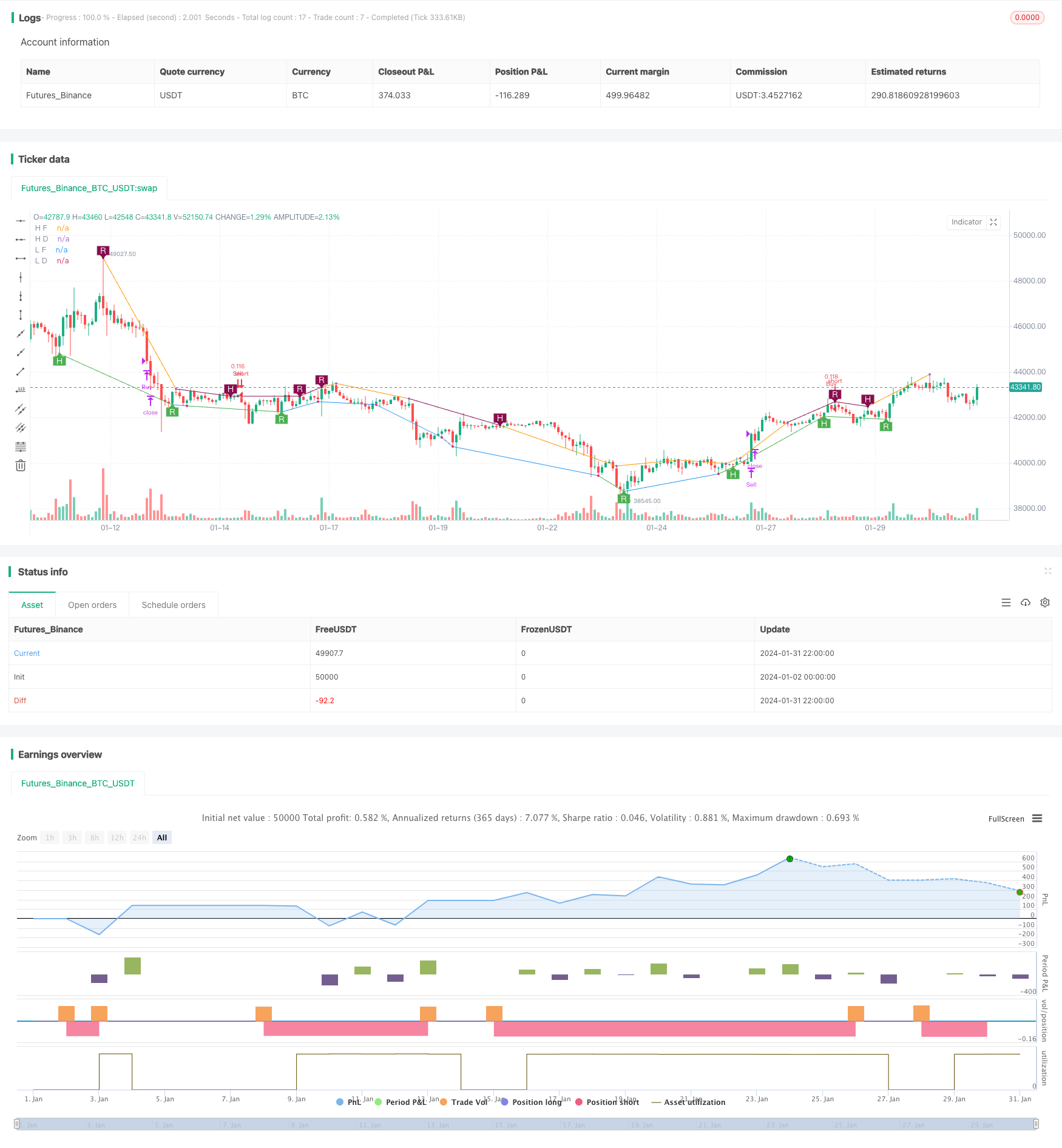
Chiến lược này là một chiến lược giao dịch theo xu hướng dựa trên tín hiệu phân tán giá. Nó sử dụng nhiều chỉ số để phát hiện tín hiệu phân tán giá, chẳng hạn như RSI, MACD, Stochastics, và xác nhận thông qua dao động Murray Math. Khi tín hiệu phân tán giá xuất hiện, nếu dao động cũng xác nhận hướng hiện tại là xu hướng, thì nhập vào.
Nguyên tắc chiến lược
Trung tâm của chiến lược này là lý thuyết phân tán giá. Khi giá sáng tạo cao nhưng chỉ số không sáng tạo cao, nó được gọi là phân tán giá thị trường gấu; khi giá sáng tạo thấp nhưng chỉ số không sáng tạo thấp, nó được gọi là phân tán giá thị trường bò. Điều này cho thấy xu hướng có thể đảo ngược.
Cụ thể, các điều kiện để tham gia chiến lược là:
- Phát hiện các tín hiệu phân tán giá, bao gồm phân tán thông thường và phân tán ẩn
- Các dao động Murrey Math nằm trong khu vực xu hướng tương ứng
Điều kiện ra sân là phẳng khi dao động quay trở lại đường trung tâm.
Phân tích lợi thế
Chiến lược này kết hợp lý thuyết phân tán giá và xác nhận xu hướng với các lợi thế sau:
- Sử dụng tín hiệu phân tán giá để phát hiện điểm đảo ngược xu hướng tiềm ẩn
- Ứng dụng dao động xác nhận xu hướng hiện tại, tránh đột phá giả
- Nhiều chỉ số và tham số kết hợp, có thể điều chỉnh linh hoạt
- Theo dõi xu hướng và tránh thua lỗ
- Các quy tắc logic rõ ràng, có nhiều không gian để tối ưu hóa mã
Phân tích rủi ro
Những rủi ro chính là:
- Các tín hiệu phân tán giá có thể là tín hiệu sai, không thể xác nhận hoàn toàn xu hướng đảo ngược
- Thiết lập tham số dao động không đúng cách có thể dẫn đến lỗ hổng và cơ hội giao dịch bị bỏ lỡ
- Tỷ lệ vị thế trống quá cao dẫn đến rủi ro mất mát lớn
- Có thể tăng số lượng giao dịch và chi phí trượt trong thời gian biến động mạnh
Đặt lệnh dừng lỗ, điều chỉnh vị trí, tối ưu hóa các tham số để giảm rủi ro.
Hướng tối ưu hóa
Chiến lược này có thể được tối ưu hóa hơn nữa:
- Thêm các thuật toán học máy để tối ưu hóa các tham số trong thời gian thực
- Thêm các kỹ thuật dừng tự điều chỉnh, như theo dõi dừng, dừng trung bình
- Kết hợp nhiều chỉ số và điều kiện lọc để tăng tỷ lệ tiếng ồn
- Động thái điều chỉnh tham số dao động, tối ưu hóa xu hướng phán đoán
- Tối ưu hóa quản lý rủi ro, thiết lập giới hạn thu hồi tối đa
Tóm tắt
Chiến lược này tích hợp lý thuyết phân tán giá và các chỉ số phân tích xu hướng để phát hiện hiệu quả các điểm chuyển hướng tiềm năng. Kết hợp với các biện pháp quản lý rủi ro tối ưu hóa, có thể đạt được tỷ lệ lợi nhuận chiến lược tốt hơn. Trong tương lai, có thể được tối ưu hóa bằng các phương pháp cao cấp như học máy để có được lợi nhuận vượt trội ổn định hơn.
/*backtest
start: 2024-01-02 00:00:00
end: 2024-02-01 00:00:00
period: 2h
basePeriod: 15m
exchanges: [{"eid":"Futures_Binance","currency":"BTC_USDT"}]
*/

//@version=2
//
// Title:   [STRATEGY][UL]Price Divergence Strategy V1
// Author:  JustUncleL
// Date:    23-Oct-2016
// Version: v1.0
//
// Description:
//  A trend trading strategy the uses Price Divergence detection signals, that
//  are confirmed by the "Murrey's Math Oscillator" (Donchanin Channel based).
//
//  *** USE AT YOUR OWN RISK ***
//
// Mofidifications:
//  1.0 - original
//
// References:
//  Strategy Based on:
//  - [RS]Price Divergence Detector V2 by RicardoSantos
//  - UCS_Murrey's Math Oscillator by Ucsgears
//  Some Code borrowed from:
//  - "Strategy Code Example by JayRogers"
//  Information on Divergence Trading:
//  - http://www.babypips.com/school/high-school/trading-divergences
//
strategy(title='[STRATEGY][UL]Price Divergence Strategy v1.0', pyramiding=0, overlay=true, initial_capital=10000, calc_on_every_tick=false,
         currency=currency.USD,default_qty_type=strategy.percent_of_equity,default_qty_value=10)
//  ||  General Input:
method = input(title='Method (0=rsi, 1=macd, 2=stoch, 3=volume, 4=acc/dist, 5=fisher, 6=cci):',  defval=1, minval=0, maxval=6)
SHOW_LABEL = input(title='Show Labels', type=bool, defval=true)
SHOW_CHANNEL = input(title='Show Channel', type=bool, defval=false)
uHid = input(true,title="Use Hidden Divergence in Strategy")
uReg = input(true,title="Use Regular Divergence in Strategy")
//  ||  RSI / STOCH / VOLUME / ACC/DIST Input:
rsi_smooth = input(title='RSI/STOCH/Volume/ACC-DIST/Fisher/cci Smooth:',  defval=5)
//  ||  MACD Input:
macd_src = input(title='MACD Source:', defval=close)
macd_fast = input(title='MACD Fast:',  defval=12)
macd_slow = input(title='MACD Slow:',  defval=26)
macd_smooth = input(title='MACD Smooth Signal:',  defval=9)
//  ||  Functions:
f_top_fractal(_src)=>_src[4] < _src[2] and _src[3] < _src[2] and _src[2] > _src[1] and _src[2] > _src[0]
f_bot_fractal(_src)=>_src[4] > _src[2] and _src[3] > _src[2] and _src[2] < _src[1] and _src[2] < _src[0]
f_fractalize(_src)=>f_top_fractal(_src) ? 1 : f_bot_fractal(_src) ? -1 : 0

//  ||••>   START MACD FUNCTION
f_macd(_src, _fast, _slow, _smooth)=>
    _fast_ma = sma(_src, _fast)
    _slow_ma = sma(_src, _slow)
    _macd = _fast_ma-_slow_ma
    _signal = ema(_macd, _smooth)
    _hist = _macd - _signal
//  ||<••   END MACD FUNCTION

//  ||••>   START ACC/DIST FUNCTION
f_accdist(_smooth)=>_return=sma(cum(close==high and close==low or high==low ? 0 : ((2*close-low-high)/(high-low))*volume), _smooth)
//  ||<••   END ACC/DIST FUNCTION

//  ||••>   START FISHER FUNCTION
f_fisher(_src, _window)=>
    _h = highest(_src, _window)
    _l = lowest(_src, _window)
    _value0 = .66 * ((_src - _l) / max(_h - _l, .001) - .5) + .67 * nz(_value0[1])
    _value1 = _value0 > .99 ? .999 : _value0 < -.99 ? -.999 : _value0
    _fisher = .5 * log((1 + _value1) / max(1 - _value1, .001)) + .5 * nz(_fisher[1])
//  ||<••   END FISHER FUNCTION

method_high = method == 0 ? rsi(high, rsi_smooth) :
  method == 1 ? f_macd(macd_src, macd_fast, macd_slow, macd_smooth) :
  method == 2 ? stoch(close, high, low, rsi_smooth) :
  method == 3 ? sma(volume, rsi_smooth) :
  method == 4 ? f_accdist(rsi_smooth) :
  method == 5 ? f_fisher(high, rsi_smooth) :
  method == 6 ? cci(high, rsi_smooth) :
  na

method_low = method == 0 ? rsi(low, rsi_smooth) :
  method == 1 ? f_macd(macd_src, macd_fast, macd_slow, macd_smooth) :
  method == 2 ? stoch(close, high, low, rsi_smooth) :
  method == 3 ? sma(volume, rsi_smooth) :
  method == 4 ? f_accdist(rsi_smooth) :
  method == 5 ? f_fisher(low, rsi_smooth) :
  method == 6 ? cci(low, rsi_smooth) :
  na

fractal_top = f_fractalize(method_high) > 0 ? method_high[2] : na
fractal_bot = f_fractalize(method_low) < 0 ? method_low[2] : na

high_prev = valuewhen(fractal_top, method_high[2], 1)
high_price = valuewhen(fractal_top, high[2], 1)
low_prev = valuewhen(fractal_bot, method_low[2], 1)
low_price = valuewhen(fractal_bot, low[2], 1)

regular_bearish_div = fractal_top and high[2] > high_price and method_high[2] < high_prev
hidden_bearish_div = fractal_top and high[2] < high_price and method_high[2] > high_prev
regular_bullish_div = fractal_bot and low[2] < low_price and method_low[2] > low_prev
hidden_bullish_div = fractal_bot and low[2] > low_price and method_low[2] < low_prev

plot(title='H F', series=fractal_top ? high[2] : na, color=regular_bearish_div or hidden_bearish_div ? maroon : not SHOW_CHANNEL ? na : silver, offset=-2)
plot(title='L F', series=fractal_bot ? low[2] : na, color=regular_bullish_div or hidden_bullish_div ? green : not SHOW_CHANNEL ? na : silver, offset=-2)
plot(title='H D', series=fractal_top ? high[2] : na, style=circles, color=regular_bearish_div or hidden_bearish_div ? maroon : not SHOW_CHANNEL ? na : silver, linewidth=3, offset=-2)
plot(title='L D', series=fractal_bot ? low[2] : na, style=circles, color=regular_bullish_div or hidden_bullish_div ? green : not SHOW_CHANNEL ? na : silver, linewidth=3, offset=-2)

plotshape(title='+RBD', series=not SHOW_LABEL ? na : regular_bearish_div ? high[2] : na, text='R', style=shape.labeldown, location=location.absolute, color=maroon, textcolor=white, offset=-2)
plotshape(title='+HBD', series=not SHOW_LABEL ? na : hidden_bearish_div ? high[2] : na, text='H', style=shape.labeldown, location=location.absolute, color=maroon, textcolor=white, offset=-2)
plotshape(title='-RBD', series=not SHOW_LABEL ? na : regular_bullish_div ? low[2] : na, text='R', style=shape.labelup, location=location.absolute, color=green, textcolor=white, offset=-2)
plotshape(title='-HBD', series=not SHOW_LABEL ? na : hidden_bullish_div ? low[2] : na, text='H', style=shape.labelup, location=location.absolute, color=green, textcolor=white, offset=-2)

// Code borrowed from UCS_Murrey's Math Oscillator by Ucsgears
//  - UCS_MMLO
// Inputs
length = input(100, minval = 10, title = "MMLO Look back Length")
quad   = input(2, minval = 1, maxval = 4, step = 1, title = "Mininum Quadrant for MMLO Support")
mult = 0.125

// Donchanin Channel
hi = highest(high, length)
lo = lowest(low, length)
range = hi - lo
multiplier = (range) * mult
midline = lo + multiplier * 4

oscillator = (close - midline)/(range/2)

a = oscillator > 0
b = oscillator > 0 and oscillator > mult*2
c = oscillator > 0 and oscillator > mult*4
d = oscillator > 0 and oscillator > mult*6

z = oscillator < 0
y = oscillator < 0 and oscillator < -mult*2
x = oscillator < 0 and oscillator < -mult*4
w = oscillator < 0 and oscillator < -mult*6


//  Strategy: (Thanks to JayRogers)
// === STRATEGY RELATED INPUTS ===
//tradeInvert     = input(defval = false, title = "Invert Trade Direction?")
// the risk management inputs
inpTakeProfit   = input(defval = 0, title = "Take Profit Points", minval = 0)
inpStopLoss     = input(defval = 0, title = "Stop Loss Points", minval = 0)
inpTrailStop    = input(defval = 100, title = "Trailing Stop Loss Points", minval = 0)
inpTrailOffset  = input(defval = 0, title = "Trailing Stop Loss Offset Points", minval = 0)

// === RISK MANAGEMENT VALUE PREP ===
// if an input is less than 1, assuming not wanted so we assign 'na' value to disable it.
useTakeProfit   = inpTakeProfit  >= 1 ? inpTakeProfit  : na
useStopLoss     = inpStopLoss    >= 1 ? inpStopLoss    : na
useTrailStop    = inpTrailStop   >= 1 ? inpTrailStop   : na
useTrailOffset  = inpTrailOffset >= 1 ? inpTrailOffset : na

// === STRATEGY - LONG POSITION EXECUTION ===
enterLong() => ((uReg and regular_bullish_div) or (uHid and hidden_bullish_div)) and (quad==1? a[1]: quad==2?b[1]: quad==3?c[1]: quad==4?d[1]: false)// functions can be used to wrap up and work out complex conditions
exitLong() => oscillator <= 0
strategy.entry(id = "Buy", long = true, when = enterLong() )// use function or simple condition to decide when to get in
strategy.close(id = "Buy", when = exitLong() )// ...and when to get out

// === STRATEGY - SHORT POSITION EXECUTION ===
enterShort() => ((uReg and regular_bearish_div) or (uHid and hidden_bearish_div)) and (quad==1? z[1]: quad==2?y[1]: quad==3?x[1]: quad==4?w[1]: false)
exitShort() => oscillator >= 0
strategy.entry(id = "Sell", long = false, when = enterShort())
strategy.close(id = "Sell", when = exitShort() )

// === STRATEGY RISK MANAGEMENT EXECUTION ===
// finally, make use of all the earlier values we got prepped
strategy.exit("Exit Buy", from_entry = "Buy", profit = useTakeProfit, loss = useStopLoss, trail_points = useTrailStop, trail_offset = useTrailOffset)
strategy.exit("Exit Sell", from_entry = "Sell", profit = useTakeProfit, loss = useStopLoss, trail_points = useTrailStop, trail_offset = useTrailOffset)


//EOF