Estratégia de acompanhamento de tendência de média móvel dinâmica de três
Visão geral
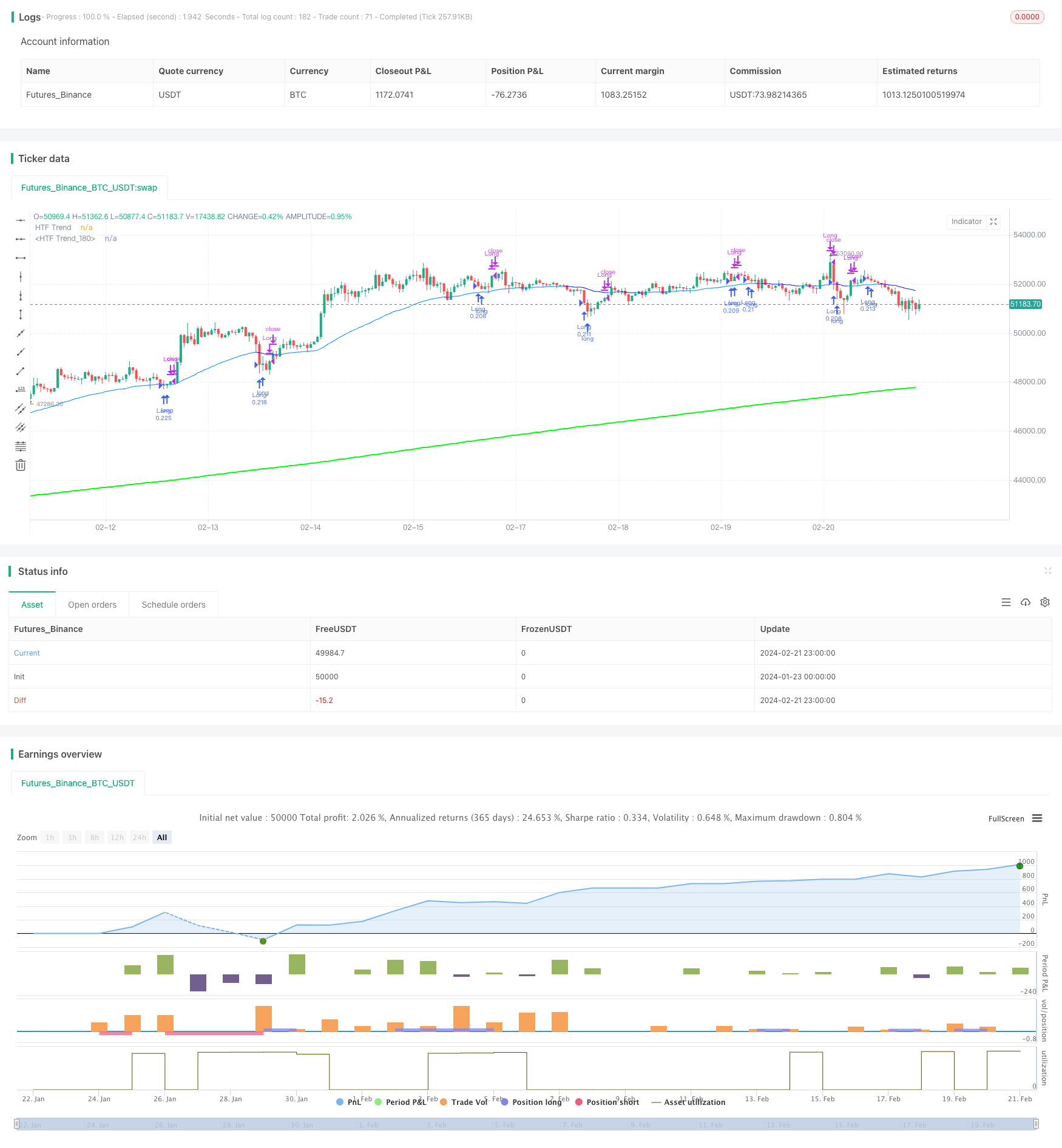
A estratégia de acompanhamento de tendências de três médias dinâmicas usa médias móveis dinâmicas e suaves em vários períodos de tempo para identificar tendências de mercado e realizar filtragem de consistência de tendências entre diferentes períodos de tempo, aumentando a confiabilidade dos sinais de negociação.
Princípio da estratégia
A estratégia usa uma dinâmica de suavização de médias móveis com três diferentes configurações de parâmetros. A primeira média móvel calcula a direção da tendência do preço do ciclo atual, a segunda média móvel calcula a direção da tendência do preço do ciclo de tempo mais alto, e a terceira média móvel calcula a direção da tendência do preço do ciclo de tempo mais alto.
As médias móveis usam a função de suavização dinâmica, que pode ser calculada automaticamente e aplicar o fator de suavização apropriado entre os diferentes períodos de tempo, permitindo que as médias móveis de períodos de tempo altos apresentem uma linha de tendência suave em um gráfico de períodos de tempo baixos, em vez de uma curva tortuosa. Esta suavização dinâmica permite que a estratégia determine a direção da tendência geral em períodos de tempo altos, enquanto executa transações em períodos de tempo baixos, permitindo um acompanhamento de tendência eficiente.
Vantagens estratégicas
A maior vantagem da estratégia reside no mecanismo de filtragem de tendências em vários períodos de tempo. Ao calcular a direção da tendência média dos preços em diferentes períodos de tempo e exigir consistência entre os diferentes períodos, é possível filtrar efetivamente a interferência de muitos tipos de flutuações de preços de curto prazo nos sinais de negociação, garantindo que cada sinal de negociação esteja dentro da grande tendência, aumentando significativamente a probabilidade de lucro.
Outra vantagem é a aplicação da função de suavização dinâmica. Isso permite que a estratégia identifique simultaneamente a tendência geral nos períodos de tempo altos e os pontos de negociação específicos nos períodos de tempo baixos. A estratégia pode determinar a direção da tendência geral nos períodos de tempo altos e executar transações específicas nos períodos de tempo baixos.
Risco e otimização
O principal risco desta estratégia é a falta de sinais de negociação. As rigorosas condições de filtragem de tendências reduzem o número de oportunidades de negociação, o que pode não ser adequado para alguns investidores que buscam negociações de alta frequência.
Além disso, a configuração de parâmetros também precisa ser cuidadosamente testada e otimizada, especialmente o comprimento de ciclo das médias móveis. Diferentes mercados precisam de configurações de parâmetros de ciclo diferentes para alcançar o melhor efeito.
A direção de otimização futura também pode considerar a adição de mais indicadores técnicos para filtragem, ou o aumento de parâmetros de otimização automática de algoritmos de aprendizado de máquina.
Resumir
Em geral, esta estratégia é uma estratégia de acompanhamento de tendências muito prática. O mecanismo de filtragem de tendências de quadros temporais múltiplos fornece um bom suporte de direção geral para cada decisão de negociação, reduzindo efetivamente o risco de negociação.
/*backtest
start: 2024-01-23 00:00:00
end: 2024-02-22 00:00:00
period: 1h
basePeriod: 15m
exchanges: [{"eid":"Futures_Binance","currency":"BTC_USDT"}]
*/

// This Pine Script™ code is subject to the terms of the Mozilla Public License 2.0 at https://mozilla.org/MPL/2.0/
// © Harrocop

//@version=5
strategy(title = "Triple MA HTF strategy - Dynamic Smoothing", shorttitle = "Triple MA strategy", overlay=true,
         pyramiding=5, initial_capital = 10000,
         calc_on_order_fills=false,
         slippage = 0,
         commission_type=strategy.commission.percent, commission_value=0.05)

//////////////////////////////////////////////////////
//////////         Risk Management        ////////////
//////////////////////////////////////////////////////
RISKM = "-------------------- Risk Management  --------------------"
InitialBalance = input.float(defval = 10000, title = "Initial Balance", minval = 1, maxval = 1000000, step = 1000, tooltip = "starting capital", group = RISKM)
LeverageEquity = input.bool(defval = true, title = "qty based on equity %", tooltip = "true turns on MarginFactor based on equity, false gives fixed qty for positionsize", group = RISKM)
MarginFactor = input.float(0, minval = - 0.9, maxval = 100, step = 0.1, tooltip = "Margin Factor, meaning that 0.5 will add 50% extra capital to determine ordersize quantity, 0.0 means 100% of equity is used to decide quantity of instrument", inline = "qty", group = RISKM)
QtyNr = input.float(defval = 3.5, title = "Quantity Contracts", minval = 0, maxval = 1000000, step = 0.01,  tooltip = "Margin Factor, meaning that 0.5 will add 50% extra capital to determine ordersize quantity, 0.0 means 100% of equity is used to decide quantity of instrument", inline = "qty", group = RISKM)
EquityCurrent = InitialBalance + strategy.netprofit[1]
QtyEquity = EquityCurrent * (1 + MarginFactor) / close[1]
QtyTrade = LeverageEquity ? QtyEquity : QtyNr

/////////////////////////////////////////////////////
//////////       MA Filter Trend         ////////////
/////////////////////////////////////////////////////
TREND = "-------------------- Moving Average 1 --------------------"
Plot_MA = input.bool(true, title = "Plot MA trend?", inline = "Trend1", group = TREND)
TimeFrame_Trend = input.timeframe(title='Higher Time Frame', defval='15', inline = "Trend1", group = TREND)
length = input.int(21, title="Length MA", minval=1, tooltip = "Number of bars used to measure trend on higher timeframe chart", inline = "Trend2", group = TREND)
MA_Type  = input.string(defval="McGinley" , options=["EMA","DEMA","TEMA","SMA","WMA", "HMA", "McGinley"], title="MA type:", inline = "Trend2", group = TREND)

ma(type, src, length) =>
    float result = 0
    if type == 'TMA' // Triangular Moving Average
        result := ta.sma(ta.sma(src, math.ceil(length / 2)), math.floor(length / 2) + 1)
        result
    if type == 'LSMA' // Least Squares Moving Average
        result := ta.linreg(src, length, 0)
        result
    if type == 'SMA'  // Simple Moving Average
        result := ta.sma(src, length)
        result
    if type == 'EMA'  // Exponential Moving Average
        result := ta.ema(src, length)
        result
    if type == 'DEMA'  // Double Exponential Moving Average
        e = ta.ema(src, length)
        result := 2 * e - ta.ema(e, length)
        result
    if type == 'TEMA'  // Triple Exponentiale
        e = ta.ema(src, length)
        result := 3 * (e - ta.ema(e, length)) + ta.ema(ta.ema(e, length), length)
        result
    if type == 'WMA'  // Weighted Moving Average
        result := ta.wma(src, length)
        result
    if type == 'HMA'  // Hull Moving Average
        result := ta.wma(2 * ta.wma(src, length / 2) - ta.wma(src, length), math.round(math.sqrt(length)))
        result
    if type == 'McGinley' // McGinley Dynamic Moving Average
        mg = 0.0
        mg := na(mg[1]) ? ta.ema(src, length) : mg[1] + (src - mg[1]) / (length * math.pow(src / mg[1], 4))
        result := mg
        result
    result

// Moving Average
MAtrend = ma(MA_Type, close, length)
MA_Value_HTF = request.security(syminfo.tickerid, TimeFrame_Trend, MAtrend)

// Get minutes for current and higher timeframes
// Function to convert a timeframe string to its equivalent in minutes
timeframeToMinutes(tf) =>
    multiplier = 1
    if (str.endswith(tf, "D"))
        multiplier := 1440
    else if (str.endswith(tf, "W"))
        multiplier := 10080
    else if (str.endswith(tf, "M"))
        multiplier := 43200
    else if (str.endswith(tf, "H"))
        multiplier := int(str.tonumber(str.replace(tf, "H", "")))
    else
        multiplier := int(str.tonumber(str.replace(tf, "m", "")))
    multiplier

// Get minutes for current and higher timeframes
currentTFMinutes = timeframeToMinutes(timeframe.period)
higherTFMinutes = timeframeToMinutes(TimeFrame_Trend)

// Calculate the smoothing factor
dynamicSmoothing = math.round(higherTFMinutes / currentTFMinutes)
MA_Value_Smooth = ta.sma(MA_Value_HTF, dynamicSmoothing)

// Trend HTF
UP = MA_Value_Smooth > MA_Value_Smooth[1] // Use "UP" Function to use as filter in combination with other indicators
DOWN = MA_Value_Smooth < MA_Value_Smooth[1] // Use "Down" Function to use as filter in combination with other indicators

/////////////////////////////////////////////////////
//////////       Second MA Filter Trend   ///////////
/////////////////////////////////////////////////////
TREND2 = "-------------------- Moving Average 2 --------------------"
Plot_MA2 = input.bool(true, title = "Plot Second MA trend?", inline = "Trend3", group = TREND2)
TimeFrame_Trend2 = input.timeframe(title='HTF', defval='60', inline = "Trend3", group = TREND2)
length2 = input.int(21, title="Length Second MA", minval=1, tooltip = "Number of bars used to measure trend on higher timeframe chart", inline = "Trend4", group = TREND2)
MA_Type2  = input.string(defval="McGinley" , options=["EMA","DEMA","TEMA","SMA","WMA", "HMA", "McGinley"], title="MA type:", inline = "Trend4", group = TREND2)

// Second Moving Average
MAtrend2 = ma(MA_Type2, close, length2)
MA_Value_HTF2 = request.security(syminfo.tickerid, TimeFrame_Trend2, MAtrend2)

// Get minutes for current and higher timeframes
higherTFMinutes2 = timeframeToMinutes(TimeFrame_Trend2)

// Calculate the smoothing factor for the second moving average
dynamicSmoothing2 = math.round(higherTFMinutes2 / currentTFMinutes)
MA_Value_Smooth2 = ta.sma(MA_Value_HTF2, dynamicSmoothing2)

// Trend HTF for the second moving average
UP2 = MA_Value_Smooth2 > MA_Value_Smooth2[1]
DOWN2 = MA_Value_Smooth2 < MA_Value_Smooth2[1]

/////////////////////////////////////////////////////
//////////       Third MA Filter Trend    ///////////
/////////////////////////////////////////////////////
TREND3 = "-------------------- Moving Average 3 --------------------"
Plot_MA3 = input.bool(true, title = "Plot third MA trend?", inline = "Trend5", group = TREND3)
TimeFrame_Trend3 = input.timeframe(title='HTF', defval='240', inline = "Trend5", group = TREND3)
length3 = input.int(50, title="Length third MA", minval=1, tooltip = "Number of bars used to measure trend on higher timeframe chart", inline = "Trend6", group = TREND3)
MA_Type3  = input.string(defval="McGinley" , options=["EMA","DEMA","TEMA","SMA","WMA", "HMA", "McGinley"], title="MA type:", inline = "Trend6", group = TREND3)

// Second Moving Average
MAtrend3 = ma(MA_Type3, close, length3)
MA_Value_HTF3 = request.security(syminfo.tickerid, TimeFrame_Trend3, MAtrend3)

// Get minutes for current and higher timeframes
higherTFMinutes3 = timeframeToMinutes(TimeFrame_Trend3)

// Calculate the smoothing factor for the second moving average
dynamicSmoothing3 = math.round(higherTFMinutes3 / currentTFMinutes)
MA_Value_Smooth3 = ta.sma(MA_Value_HTF3, dynamicSmoothing3)

// Trend HTF for the second moving average
UP3 = MA_Value_Smooth3 > MA_Value_Smooth3[1]
DOWN3 = MA_Value_Smooth3 < MA_Value_Smooth3[1]

/////////////////////////////////////////////////////
//////////         Entry Settings        ////////////
/////////////////////////////////////////////////////
BuySignal = ta.crossover(MA_Value_HTF, MA_Value_HTF2) and UP3 == true
SellSignal = ta.crossunder(MA_Value_HTF, MA_Value_HTF2) and DOWN3 == true
ExitBuy = ta.crossunder(MA_Value_HTF, MA_Value_HTF2)
ExitSell = ta.crossover(MA_Value_HTF, MA_Value_HTF2)

/////////////////////////////////////////////////
///////////       Strategy       ////////////////
///////////      Entry & Exit    ////////////////
///////////         logic        ////////////////
/////////////////////////////////////////////////
// Long
if BuySignal
    strategy.entry("Long", strategy.long, qty = QtyTrade)

if (strategy.position_size > 0 and ExitBuy == true)
    strategy.close(id = "Long", comment = "Close Long")

// Short
if SellSignal
    strategy.entry("Short", strategy.short, qty = QtyTrade)

if (strategy.position_size < 0 and ExitSell == true)
    strategy.close(id = "Short", comment = "Close Short")

/////////////////////////////////////////////////////
//////////         Visuals Chart         ////////////
/////////////////////////////////////////////////////
// Plot Moving Average HTF
p1 = plot(Plot_MA ? MA_Value_Smooth : na, "HTF Trend", color = UP ? color.rgb(238, 255, 0) : color.rgb(175, 173, 38), linewidth = 1, style = plot.style_line)
p2 = plot(Plot_MA2 ? MA_Value_Smooth2 : na, "HTF Trend", color = UP2 ? color.rgb(0, 132, 255) : color.rgb(0, 17, 255), linewidth = 1, style = plot.style_line)
plot(Plot_MA3 ? MA_Value_Smooth3 : na, "HTF Trend", color = UP3 ? color.rgb(0, 255, 8) : color.rgb(255, 0, 0), linewidth = 2, style = plot.style_line)
fill(p1, p2, color = color.rgb(255, 208, 0, 90), title="Fill")