Chiến lược theo dõi xu hướng đa dòng thời gian
Tổng quan
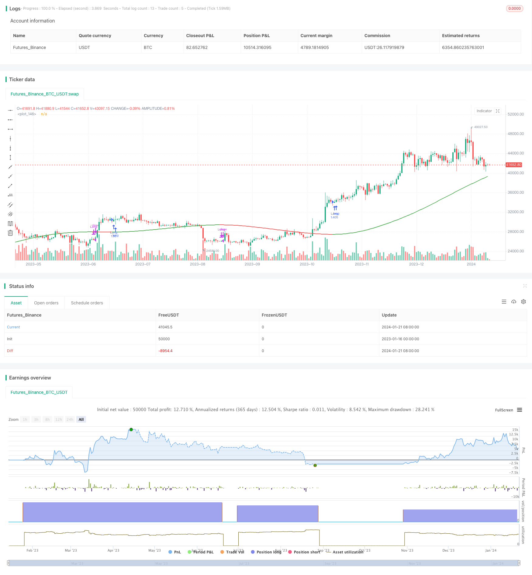
Chiến lược theo dõi xu hướng đa thời gian là một chiến lược theo dõi xu hướng kết hợp nhiều đường trung bình di chuyển và đường hồi phục khác nhau. Chiến lược này có thể lựa chọn trong hơn 20 chỉ số xu hướng khác nhau để thực hiện mua và bán tự động.
Nguyên tắc chiến lược
Trọng tâm của chiến lược này là để xác định xem giá có đang tăng hay giảm dựa trên các chỉ số xu hướng mà người dùng chọn. Chiến lược này đầu tiên tính toán hơn 20 đường trung bình di chuyển và đường hồi phục. Những chỉ số này bao gồm các chỉ số trong thư viện tiêu chuẩn ngôn ngữ lập trình Pine như trung bình di chuyển thông thường, trung bình di chuyển có trọng lượng và trung bình di chuyển chỉ số, cũng bao gồm một số chỉ số tùy chỉnh được viết bởi cộng đồng Pine.
Phân tích lợi thế
Chiến lược này kết hợp hơn 20 xu hướng đánh giá chỉ số, tránh khả năng đánh giá sai lầm chỉ số duy nhất. Và các chỉ số này đã được xác minh bởi các nhà phát triển cộng đồng. Có thể điều chỉnh bằng các tham số khác nhau và áp dụng cho nhiều môi trường thị trường.
So với chiến lược trung bình di chuyển đôi đơn giản, chiến lược này chỉ dựa vào một chỉ số để xác định xu hướng, thể hiện xu hướng tốt hơn và không có tín hiệu sai trái trái với chỉ số.
Phân tích rủi ro
Chiến lược này phụ thuộc vào các chỉ số để đánh giá xu hướng và không thể xác định xu hướng đã bị đảo ngược. Do đó, sẽ có một mức độ chậm trễ. Điều này có thể dẫn đến tổn thất hoặc bỏ lỡ cơ hội.
Sau khi xảy ra sự kiện bất ngờ, tất cả các chiến lược theo xu hướng sẽ tạo ra tổn thất lớn. Cần thiết lập lỗ dừng để kiểm soát rủi ro.
Hướng tối ưu hóa
Có thể xem xét kết hợp với các chỉ số khác để dự đoán sự đảo ngược xu hướng để giảm thiểu các vấn đề về sự chậm trễ. Ví dụ, kết hợp với chỉ số Brin để xác định liệu giá có mở rộng quá mức hay không.
Có thể thiết kế cơ chế dừng lỗ khẩn cấp cho các sự kiện bất ngờ. Ví dụ: bắt buộc dừng lỗ khi xảy ra tổn thất hơn 5% trong một ngày.
Tóm tắt
Chiến lược theo dõi xu hướng đa thời gian kết hợp hơn 20 chỉ số đánh giá xu hướng, thể hiện đầy đủ xu hướng thị trường, tránh tín hiệu sai. Trong khi vẫn có khả năng tùy chỉnh cao, có thể áp dụng cho môi trường thị trường có sự khác biệt lớn. Đây là một chiến lược theo dõi xu hướng rất hiệu quả. Bằng cách thiết lập các thông số chỉ số dừng và tối ưu hóa thích hợp, có thể nhận được lợi nhuận tốt hơn với điều kiện kiểm soát rủi ro.
/*backtest
start: 2023-01-16 00:00:00
end: 2024-01-22 00:00:00
period: 1d
basePeriod: 1h
exchanges: [{"eid":"Futures_Binance","currency":"BTC_USDT"}]
*/

// This source code is subject to the terms of the Mozilla Public License 2.0 at https://mozilla.org/MPL/2.0/
// @version=5
// Author = TradeAutomation


strategy(title="Multi MA Trend Following Strategy Template", shorttitle="Multi Trend", process_orders_on_close=true, overlay=true, commission_type=strategy.commission.cash_per_order, commission_value=1, slippage = 0, margin_short = 75, margin_long = 75, initial_capital = 100000000, default_qty_type=strategy.percent_of_equity, default_qty_value=100)

// Backtest Date Range Inputs //
StartTime = input(defval=timestamp('01 Jan 2019 05:00 +0000'), group="Date Rangte", title='Start Time')
EndTime = input(defval=timestamp('01 Jan 2099 00:00 +0000'), group="Date Range", title='End Time')
InDateRange = true

// Trend Selector //
TrendSelectorInput = input.string(title="Trend Selector", defval="JMA", group="Core Settings", options=["ALMA", "DEMA", "EMA", "HMA", "JMA", "KAMA", "Linear Regression (LSMA)", "RMA", "SMA", "SMMA", "Source", "SuperTrend", "TEMA", "TMA", "VAMA", "VIDYA", "VMA", "VWMA", "WMA", "WWMA", "ZLEMA"], tooltip="Select your moving average")
src = input.source(close, "Source", group="Core Settings", tooltip="This is the price source being used for the moving averages to calculate based on")
length = input.int(200, "MA Length", group="Core Settings", tooltip="This is the amount of historical bars being used for the moving averages to calculate based on")
LineWidth = input.int(2, "Line Width", group="Core Settings", tooltip="This is the width of the line plotted that represents the selected trend")

// Individual Moving Average / Regression Setting //
AlmaOffset = input.float(0.85, "ALMA Offset", group="Individual MA Settings", tooltip="This only applies when ALMA is selected")
AlmaSigma = input.float(6, "ALMA Sigma", group="Individual MA Settings", tooltip="This only applies when ALMA is selected")
ATRFactor = input.float(3, "ATR Multiplier For SuperTrend", group="Individual MA Settings", tooltip="This only applies when SuperTrend is selected")
ATRLength = input.int(12, "ATR Length For SuperTrend", group="Individual MA Settings", tooltip="This only applies when SuperTrend is selected")
JMApower = input.int(2, "JMA Power Parameter", group="Individual MA Settings", tooltip="This only applies when JMA is selected")
KamaAlpha = input.float(3, "KAMA's Alpha", minval=1,step=0.5, group="Individual MA Settings", tooltip="This only applies when KAMA is selected")
LinRegOffset = input.int(0, "Linear Regression Offset", group="Individual MA Settings", tooltip="This only applies when Linear Regression is selected")
VAMALookback =input.int(12, "VAMA Volatility lookback", group="Individual MA Settings", tooltip="This only applies when VAMA is selected")

// Trend Indicators in Library //
ALMA = ta.alma(src, length, AlmaOffset, AlmaSigma)
EMA = ta.ema(src, length)
HMA = ta.hma(src, length)
LinReg = ta.linreg(src, length, LinRegOffset)
RMA = ta.rma(src, length)
SMA = ta.sma(src, length)
VWMA = ta.vwma(src, length)
WMA = ta.wma(src, length)

// Additional Trend Indicators Written and/or Open Sourced //
//DEMA
de1 = ta.ema(src, length)
de2 = ta.ema(de1, length)
DEMA = 2 * de1 - de2

//JMA [Capissmo]
beta = 0.45*(length-1)/(0.45*(length-1)+2)
alpha = math.pow(beta, JMApower)
L0=0.0, L1=0.0, L2=0.0, L3=0.0, JMA=0.0
L0 := (1-alpha)*src + alpha*nz(L0[1])
L1 := (src - L0[0])*(1-beta) + beta*nz(L1[1])
L2 := L0[0] + L1[0]
L3 := (L2[0] - nz(JMA[1]))*((1-alpha)*(1-alpha)) + (alpha*alpha)*nz(L3[1])
JMA := nz(JMA[1]) + L3[0]

//KAMA
var KAMA = 0.0
fastAlpha = 2.0 / (KamaAlpha + 1)
slowAlpha = 2.0 / 31
momentum = math.abs(ta.change(src, length))
volatility = math.sum(math.abs(ta.change(src)), length)
efficiencyRatio = volatility != 0 ? momentum / volatility : 0
smoothingConstant = math.pow((efficiencyRatio * (fastAlpha - slowAlpha)) + slowAlpha, 2)
KAMA := nz(KAMA[1], src) + smoothingConstant * (src - nz(KAMA[1], src))

//SMMA
var SMMA = 0.0
SMMA := na(SMMA[1]) ? ta.sma(src, length) : (SMMA[1] * (length - 1) + src) / length

//SuperTrend
ATR = ta.atr(ATRLength)
Signal = ATRFactor*ATR
var SuperTrend = 0.0
SuperTrend := if src>SuperTrend[1] and src[1]>SuperTrend[1]
    math.max(SuperTrend[1], src-Signal)
else if src<SuperTrend[1] and src[1]<SuperTrend[1]
    math.min(SuperTrend[1], src+Signal)
else if src>SuperTrend[1]
    src-Signal
else
    src+Signal

//TEMA
t1 = ta.ema(src, length)
t2 = ta.ema(t1, length)
t3 = ta.ema(t2, length)
TEMA = 3 * (t1 - t2) + t3

//TMA
TMA = ta.sma(ta.sma(src, math.ceil(length / 2)), math.floor(length / 2) + 1)

//VAMA
mid=ta.ema(src,length)
dev=src-mid
vol_up=ta.highest(dev,VAMALookback)
vol_down=ta.lowest(dev,VAMALookback)
VAMA = mid+math.avg(vol_up,vol_down)

//VIDYA [KivancOzbilgic]
var VIDYA=0.0
VMAalpha=2/(length+1)
ud1=src>src[1] ? src-src[1] : 0
dd1=src<src[1] ? src[1]-src : 0
UD=math.sum(ud1,9)
DD=math.sum(dd1,9)
CMO=nz((UD-DD)/(UD+DD))
VIDYA := na(VIDYA[1]) ? ta.sma(src, length) : nz(VMAalpha*math.abs(CMO)*src)+(1-VMAalpha*math.abs(CMO))*nz(VIDYA[1])

//VMA [LazyBear]
sc = 1/length
pdm = math.max((src - src[1]), 0)
mdm = math.max((src[1] - src), 0)
var pdmS = 0.0
var mdmS = 0.0
pdmS := ((1 - sc)*nz(pdmS[1]) + sc*pdm)
mdmS := ((1 - sc)*nz(mdmS[1]) + sc*mdm)
s = pdmS + mdmS
pdi = pdmS/s
mdi = mdmS/s
var pdiS = 0.0
var mdiS = 0.0
pdiS := ((1 - sc)*nz(pdiS[1]) + sc*pdi)
mdiS := ((1 - sc)*nz(mdiS[1]) + sc*mdi)
d = math.abs(pdiS - mdiS)
s1 = pdiS + mdiS
var iS = 0.0
iS := ((1 - sc)*nz(iS[1]) + sc*d/s1)
hhv = ta.highest(iS, length)
llv = ta.lowest(iS, length)
d1 = hhv - llv
vi = (iS - llv)/d1
var VMA=0.0
VMA := sc*vi*src + (1 - sc*vi)*nz(VMA[1])

//WWMA
var WWMA=0.0
WWMA := (1/length)*src + (1-(1/length))*nz(WWMA[1])

//Zero Lag EMA
EMA1 = ta.ema(src,length)
EMA2 = ta.ema(EMA1,length)
Diff = EMA1 - EMA2
ZLEMA = EMA1 + Diff

// Trend Mapping and Plotting //
Trend = TrendSelectorInput == "ALMA" ? ALMA : TrendSelectorInput == "DEMA" ? DEMA : TrendSelectorInput == "EMA" ? EMA : TrendSelectorInput == "HMA" ? HMA : TrendSelectorInput == "JMA" ? JMA : TrendSelectorInput == "KAMA" ? KAMA : TrendSelectorInput == "Linear Regression (LSMA)" ? LinReg : TrendSelectorInput == "RMA" ? RMA : TrendSelectorInput == "SMA" ? SMA : TrendSelectorInput == "SMMA" ? SMMA : TrendSelectorInput == "Source" ? src : TrendSelectorInput == "SuperTrend" ? SuperTrend : TrendSelectorInput == "TEMA" ? TEMA : TrendSelectorInput == "TMA" ? TMA : TrendSelectorInput == "VAMA" ? VAMA : TrendSelectorInput == "VIDYA" ? VIDYA : TrendSelectorInput == "VMA" ? VMA : TrendSelectorInput == "VWMA" ? VWMA : TrendSelectorInput == "WMA" ? WMA : TrendSelectorInput == "WWMA" ? WWMA : TrendSelectorInput == "ZLEMA" ? ZLEMA : SMA
plot(Trend, color=(Trend>Trend[1]) ? color.green : (Trend<Trend[1]) ? color.red : (Trend==Trend[1]) ? color.gray : color.black, linewidth=LineWidth)

// Entry & Exit Functions //

if (InDateRange)
    strategy.entry("Long", strategy.long, when = ta.crossover(Trend, Trend[1]))
    strategy.close("Long", when = ta.crossunder(Trend, Trend[1]))
if (not InDateRange)
    strategy.close_all()