
La idea principal de esta estrategia es identificar la dirección de la tendencia en un marco de tiempo más grande y encontrar un punto de entrada de ruptura en un marco de tiempo más pequeño, mientras que el stop loss exit sigue la media móvil en un marco de tiempo más grande.
La estrategia se basa principalmente en tres indicadores:
En primer lugar, se calcula un promedio móvil simple de X días de un período más largo (como la línea de sol) y se permite comprar solo cuando el promedio móvil está en la estación de precios. Esto puede usarse para determinar la dirección de la tendencia general y evitar períodos de volatilidad en el comercio.
En segundo lugar, se calcula el máximo precio de un período más corto (por ejemplo, 5 días) Swing High, cuando el precio se rompe el máximo precio se activa la señal de compra. Aquí se combina con una revisión del parámetro de ciclo lb para encontrar el punto de ruptura adecuado.
En tercer lugar, establezca una línea de parada. Una vez en posición, la línea de parada se bloquea en el precio mínimo de un determinado período de lbStop a la distancia del punto más bajo más reciente. Al mismo tiempo, establezca un promedio móvil (como la línea solar 10 días de EMA) como mecanismo de salida, y salga de la posición cuando el precio esté por debajo de ese promedio móvil.
La estrategia también establece un valor de ATR para evitar la compra de puntos exagerados. Además, hay otras condiciones auxiliares como el rango de tiempo de retracción.
La interacción de estos tres indicadores constituye la lógica central de la estrategia.
Esta es una estrategia de tipo de seguimiento de brecha que tiene las siguientes ventajas:
Utiliza dos marcos de tiempo para evitar estar atrapado en falsas rupturas de mercados convulsivos. El marco de tiempo más largo para juzgar la tendencia general, el marco de tiempo más corto para buscar puntos de entrada específicos.
Utilizando los puntos de ruptura que se forman en el swing high, este tipo de ruptura tiene cierta inercia y es fácil de seguir. Al mismo tiempo, se puede ajustar el parámetro de revisión del ciclo lb para buscar una ruptura realmente efectiva.
El método de stop loss es más riguroso, ya que se rastrea el punto más bajo más reciente y se deja una cierta distancia de amortiguamiento para evitar que se bloquee.
El uso de la media móvil como mecanismo de salida permite una suspensión flexible según las circunstancias.
El indicador ATR evita los riesgos de una emisión excesiva.
Se pueden configurar diferentes combinaciones de parámetros para probar el efecto, con un mayor espacio de optimización.
La estrategia también tiene ciertos riesgos:
Cuando los precios oscilan hacia arriba y hacia abajo cerca de las medias móviles, es fácil ser cambiado de posición de entrada y salida repetidamente. En este caso, se enfrenta al riesgo de comisiones más altas.
Cuando se rompe el punto de compra cerca de la media móvil, existe un mayor riesgo de retiro. Esto es una característica de la estrategia misma.
Cuando no hay una tendencia evidente, el tiempo de mantenimiento de la posición puede ser demasiado largo y se enfrenta a un riesgo de tiempo.
Es necesario ajustar razonablemente los parámetros de ATR. Si el ATR es demasiado pequeño, el filtro es más débil, y si es demasiado grande, la oportunidad de entrada es menor.
Se necesita probar el efecto de los diferentes parámetros lb en los resultados. Parámetros demasiado grandes pueden perder algunas oportunidades, y los parámetros demasiado pequeños pueden identificar falsos avances.
La solución al riesgo:
La estrategia también se puede optimizar en las siguientes dimensiones:
Prueba diferentes combinaciones de parámetros de la media móvil para encontrar el parámetro óptimo.
Prueba diferentes configuraciones de parámetros ATR para equilibrar las oportunidades de ingreso y el control de riesgos.
Optimización de los parámetros de retrospectiva del ciclo lb para identificar brechas más eficientes.
Intentar establecer un stop loss dinámico para controlar el riesgo en función de la volatilidad y el retiro.
La efectividad de la brecha se determina en combinación con otros factores, como el indicador de volumen de transacciones.
Desarrollar métodos de búsqueda de puntos extremos como referencia, como por ejemplo </‘,</,><
Intentar entrenar a los parámetros con el aprendizaje automático para obtener el parámetro óptimo
La estrategia en su conjunto es una estrategia de seguimiento de brecha típica. El juicio de doble marco de tiempo, el Swing High identifica el momento de entrada, la línea de parada y el mecanismo de salida de doble seguro de la media móvil, formando un sistema lógico completo. La estrategia tiene características de riesgo y ganancia más claras y es adecuada para el tipo de inversor que sigue la línea media y larga. Aunque existe un cierto riesgo, se puede reducir el nivel de riesgo mediante la optimización de parámetros y la optimización de reglas.
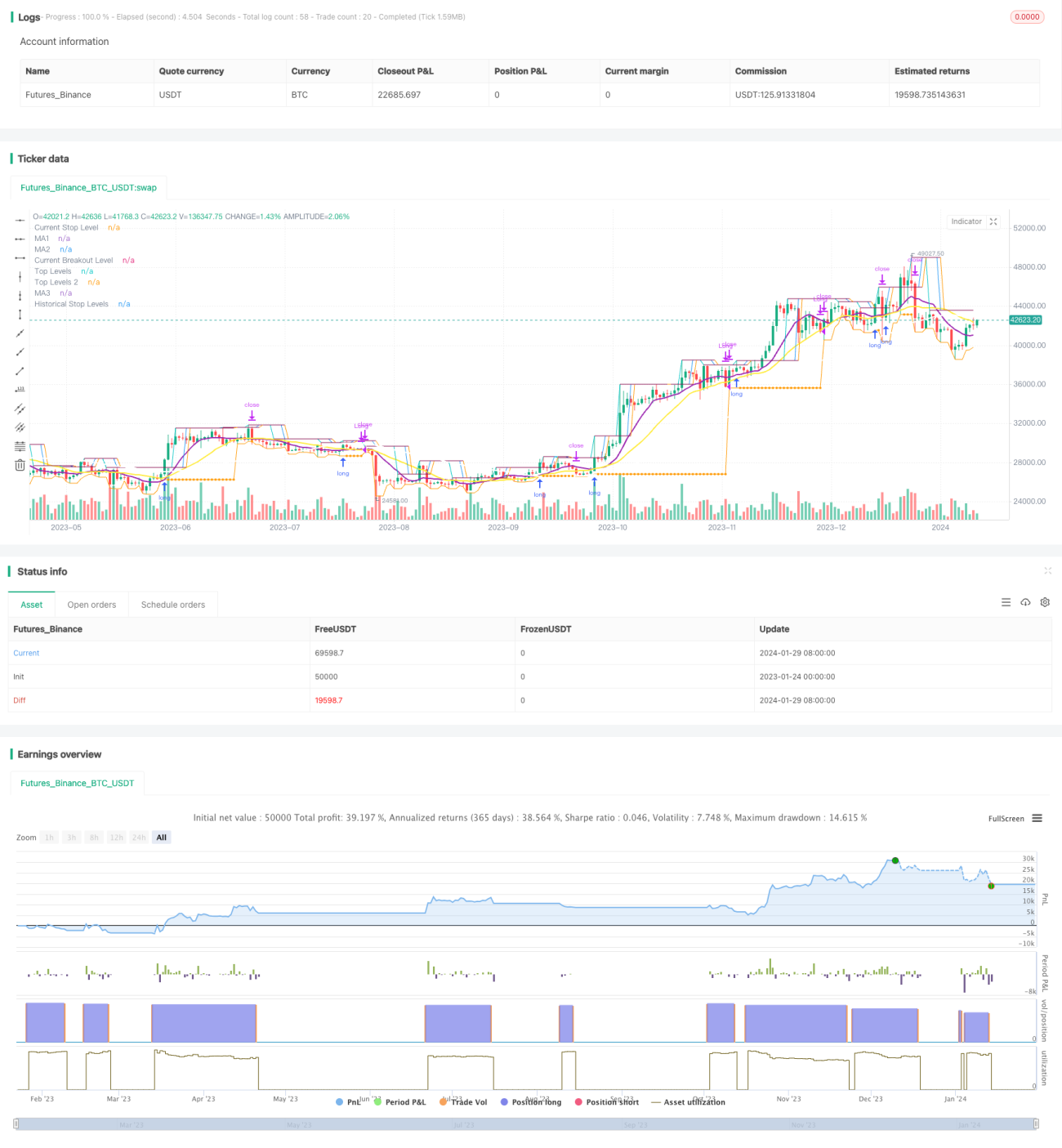
/*backtest
start: 2023-01-24 00:00:00
end: 2024-01-30 00:00:00
period: 1d
basePeriod: 1h
exchanges: [{"eid":"Futures_Binance","currency":"BTC_USDT"}]
*/
// This source code is subject to the terms of the Mozilla Public License 2.0 at https://mozilla.org/MPL/2.0/
// © millerrh
// The intent of this strategy is to buy breakouts with a tight stop on smaller timeframes in the direction of the longer term trend.
// Then use a trailing stop of a close below either the 10 MA or 20 MA (user choice) on that larger timeframe as the position
// moves in your favor (i.e. whenever position price rises above the MA).
// Option of using daily ATR as a measure of finding contracting ranges and ensuring a decent risk/reward.
// (If the difference between the breakout point and your stop level is below a certain % of ATR, it could possibly find those consolidating periods.)
//@version=4
strategy("Qullamaggie Breakout", overlay=true, initial_capital=10000, currency='USD',
default_qty_type=strategy.percent_of_equity, default_qty_value=100, commission_type=strategy.commission.percent, commission_value=0.1)
// === BACKTEST RANGE ===
Start = input(defval = timestamp("01 Jan 2019 06:00 +0000"), title = "Backtest Start Date", type = input.time)
Finish = input(defval = timestamp("01 Jan 2100 00:00 +0000"), title = "Backtest End Date", type = input.time)
// Inputs
lb = input(defval = 3, title = "Lookback Period for Swing High", minval = 1,
tooltip = "Lookback period for defining the breakout level.")
lbStop = input(defval = 3, title = "Lookback Bars for Stop Level", minval = 1,
tooltip = "Initial stop placement is the lowest low this many bars back. Allows for tighter stop placement than referencing swing lows.")
htf = input(defval="D", title="Timeframe of Moving Averages", type=input.resolution,
tooltip = "Allows you to set a different time frame for the moving averages. The default behavior is to identify good tightening setups on a larger timeframe
(like daily) and enter the trade on a breakout occuring on a smaller timeframe, using the moving averages of the larger timeframe to trail your stop.")
maType = input(defval="SMA", options=["EMA", "SMA"], title = "Moving Average Type")
ma1Length = input(defval = 10, title = "1st Moving Average Length", minval = 1)
ma2Length = input(defval = 20, title = "2nd Moving Average Length", minval = 1)
ma3Length = input(defval = 50, title = "3rd Moving Average Length", minval = 1)
useMaFilter = input(title = "Use 3rd Moving Average for Filtering?", type = input.bool, defval = true,
tooltip = "Signals will be ignored when price is under this slowest moving average. The intent is to keep you out of bear periods and only
buying when price is showing strength or trading with the longer term trend.")
trailMaInput = input(defval="2nd Moving Average", options=["1st Moving Average", "2nd Moving Average"], title = "Trailing Stop")
// MA Calculations
ma(maType, src, length) =>
maType == "EMA" ? ema(src, length) : sma(src, length) //Ternary Operator (if maType equals EMA, then do ema calc, else do sma calc)
ma1 = security(syminfo.tickerid, htf, ma(maType, close, ma1Length))
ma2 = security(syminfo.tickerid, htf, ma(maType, close, ma2Length))
ma3 = security(syminfo.tickerid, htf, ma(maType, close, ma3Length))
plot(ma1, color=color.purple, style=plot.style_line, title="MA1", linewidth=2, transp = 60)
plot(ma2, color=color.yellow, style=plot.style_line, title="MA2", linewidth=2, transp = 60)
plot(ma3, color=color.white, style=plot.style_line, title="MA3", linewidth=2, transp = 60)
// === USE ATR FOR FILTERING ===
// The idea here is that you want to buy in a consolodating range for best risk/reward. So here you can compare the current distance between
// support/resistance vs.the ATR and make sure you aren't buying at a point that is too extended from normal.
useAtrFilter = input(title = "Use ATR for Filtering?", type = input.bool, defval = false,
tooltip = "Signals will be ignored if the distance between support and resistance is larger than a user-defined percentage of Daily ATR.
This allows the user to ensure they are not buying something that is too extended and instead focus on names that are consolidating more.")
atrPerc = input(defval = 100, title = "% of Daily ATR Value", minval = 1)
atrValue = security(syminfo.tickerid, "D", atr(14))*atrPerc*.01
// === PLOT SWING HIGH/LOW AND MOST RECENT LOW TO USE AS STOP LOSS EXIT POINT ===
// Change these values to adjust the look back and look forward periods for your swing high/low calculations
pvtLenL = lb
pvtLenR = lb
// Get High and Low Pivot Points
pvthi_ = pivothigh(high, pvtLenL, pvtLenR)
pvtlo_ = pivotlow(low, pvtLenL, pvtLenR)
// Force Pivot completion before plotting.
Shunt = 1 //Wait for close before printing pivot? 1 for true 0 for flase
maxLvlLen = 0 //Maximum Extension Length
pvthi = pvthi_[Shunt]
pvtlo = pvtlo_[Shunt]
// Count How many candles for current Pivot Level, If new reset.
counthi = barssince(not na(pvthi))
countlo = barssince(not na(pvtlo))
pvthis = fixnan(pvthi)
pvtlos = fixnan(pvtlo)
hipc = change(pvthis) != 0 ? na : color.maroon
lopc = change(pvtlos) != 0 ? na : color.green
// Display Pivot lines
plot((maxLvlLen == 0 or counthi < maxLvlLen) ? pvthis : na, color=hipc, transp=0, linewidth=1, offset=-pvtLenR-Shunt, title="Top Levels")
// plot((maxLvlLen == 0 or countlo < maxLvlLen) ? pvtlos : na, color=lopc, transp=0, linewidth=1, offset=-pvtLenR-Shunt, title="Bottom Levels")
plot((maxLvlLen == 0 or counthi < maxLvlLen) ? pvthis : na, color=hipc, transp=0, linewidth=1, offset=0, title="Top Levels 2")
// plot((maxLvlLen == 0 or countlo < maxLvlLen) ? pvtlos : na, color=lopc, transp=0, linewidth=1, offset=0, title="Bottom Levels 2")
// BUY CONDITIONS
stopLevelCalc = valuewhen(pvtlo_, low[pvtLenR], 0) //Stop Level at Swing Low
buyLevel = valuewhen(pvthi_, high[pvtLenR], 0) //Buy level at Swing High
plot(buyLevel, style=plot.style_line, color=color.blue, title = "Current Breakout Level", show_last=1, linewidth=1, transp=50, trackprice=true)
// Conditions for entry and exit
stopLevel = float(na) // Define stop level here as "na" so that I can reference it in the inPosition
// variable and the ATR calculation before the stopLevel is actually defined.
buyConditions = (useMaFilter ? buyLevel > ma3 : true) and
(useAtrFilter ? (buyLevel - stopLevel[1]) < atrValue : true)
// buySignal = high > buyLevel and buyConditions
buySignal = crossover(high, buyLevel) and buyConditions
trailMa = trailMaInput == "1st Moving Average" ? ma1 : ma2
sellSignal = crossunder(close, trailMa)
// sellSignal = security(syminfo.tickerid, htf, close < trailMa) and security(syminfo.tickerid, htf, close[1] < trailMa)
// STOP AND PRICE LEVELS
inPosition = bool(na)
inPosition := buySignal[1] ? true : sellSignal[1] ? false : low <= stopLevel[1] ? false : inPosition[1]
lowDefine = lowest(low, lbStop)
stopLevel := inPosition ? stopLevel[1] : lowDefine
// plot(stopLevel)
buyPrice = buyLevel
buyPrice := inPosition ? buyPrice[1] : buyLevel
plot(stopLevel, style=plot.style_line, color=color.orange, title = "Current Stop Level", show_last=1, linewidth=1, transp=50, trackprice=true)
plot(inPosition ? stopLevel : na, style=plot.style_circles, color=color.orange, title = "Historical Stop Levels", transp=50, trackprice=false)
// plot(buyPrice, style=plot.style_line, color=color.blue, linewidth=1, transp=50, trackprice=true)
// (STRATEGY ONLY) Comment out for Study
strategy.entry("Long", strategy.long, stop = buyLevel, when = buyConditions)
strategy.exit("Exit Long", from_entry = "Long", stop=stopLevel[1])
if (low[1] > trailMa)
strategy.close("Long", when = sellSignal)
// if (low[1] > trailMa)
// strategy.exit("Exit Long", from_entry = "Long", stop=trailMa) //to get this to work right, I need to reference highest highs instead of swing highs
//because it can have me buy right back in after selling if the stop level is above the last registered swing high point.