Estratégia de rastreamento de fuga de Qullamaggie

Autora:ChaoZhang, Data: 2024-01-31 17:06:36
Tags:

Resumo

A ideia principal desta estratégia é identificar a direção da tendência em um período de tempo maior e encontrar pontos de ruptura para entrar em um período de tempo menor.

Princípio da estratégia

Esta estratégia baseia-se principalmente em três indicadores de avaliação.

Primeiro, calcule um ciclo mais longo (como diário) média móvel simples de X dias. Permita comprar apenas quando o preço estiver acima desta média móvel. Isso pode ser usado para determinar a direção geral da tendência e evitar períodos de negociação oscilantes.

Em segundo lugar, calcule o preço mais alto Swing High em um ciclo mais curto (como 5 dias). Quando o preço atravessa esse preço mais alto, um sinal de compra é acionado.

Terceiro, estabeleça uma linha de stop loss. Após entrar na posição, a linha de stop loss é bloqueada no preço mais baixo um certo período de tempo lbStop longe do ponto mais baixo recente. Ao mesmo tempo, defina uma linha média móvel (como a EMA de 10 dias no diário) como um mecanismo de saída. Saia da posição quando o preço estiver abaixo desta linha média móvel.

A estratégia também define o valor ATR para evitar a compra de pontos sobre-extendidos.

O julgamento da interacção dos três indicadores acima é a lógica central desta estratégia.

Análise das vantagens

Como estratégia de rastreamento de fuga, tem as seguintes vantagens:

Use dois prazos para evitar ser preso em falhas de ruptura em mercados oscilantes. O prazo mais longo determina a tendência geral e o prazo mais curto encontra pontos de entrada específicos.
Este tipo de ruptura tem certa inércia e é fácil de formar rastreamento. O parâmetro de período de olho de lb também pode ser ajustado para encontrar rupturas verdadeiramente eficazes.
O método de stop loss é relativamente rigoroso, acompanhando o ponto mais baixo recente com uma certa distância de amortecimento para evitar ser raspado.
Usar a média móvel como mecanismo de saída para obter lucros de forma flexível de acordo com as condições do mercado.
O indicador ATR evita o risco de alavancagem excessiva.
Diferentes combinações de parâmetros podem ser definidas para testes, com grande espaço de otimização.

Análise de riscos

A estratégia apresenta também alguns riscos:

Quando o preço oscila para cima e para baixo em torno da linha da média móvel, é fácil alternar para frente e para trás entre as posições de entrada e saída.
Quando o ponto de ruptura está próximo da linha da média móvel, há um risco de retração relativamente grande.
Quando não há uma tendência óbvia no mercado, o tempo de detenção pode ser demasiado longo, enfrentando um risco temporal.
O parâmetro ATR precisa ser definido de forma razoável. Se o ATR for muito pequeno, o efeito de filtragem é fraco. Se for muito grande, as oportunidades de entrada diminuirão.
A necessidade de testar o impacto de diferentes parâmetros de lb nos resultados. Parâmetros excessivamente grandes podem perder algumas oportunidades, enquanto parâmetros muito pequenos podem identificar falhas.

Mitigação do risco:

Ajustar adequadamente os parâmetros da média móvel para aumentar a capacidade de filtragem.
Otimizar os parâmetros do ATR, complementados pelo julgamento visual.
Ajuste o período de observação para encontrar os parâmetros ideais.
Suspenda a negociação durante os mercados osciladores.

Orientações de otimização

A estratégia pode também ser otimizada nas seguintes dimensões:

Teste diferentes combinações de parâmetros da média móvel para encontrar os parâmetros ideais.
Tente diferentes configurações de parâmetros ATR para equilibrar as oportunidades de entrada e o controlo de riscos.
Otimizar o parâmetro do período de observação de lb para identificar breakouts mais eficientes.
Tente criar um stop loss dinâmico baseado na volatilidade e no drawdown para controlar o risco.
Incorporar outros fatores, tais como o volume de negociação, para determinar a eficácia dos breakouts.
Desenvolver/,< e outros métodos para encontrar pontos extremos como referências.
Tente Machine Learning para treinar parâmetros para parâmetros ideais

Resumo

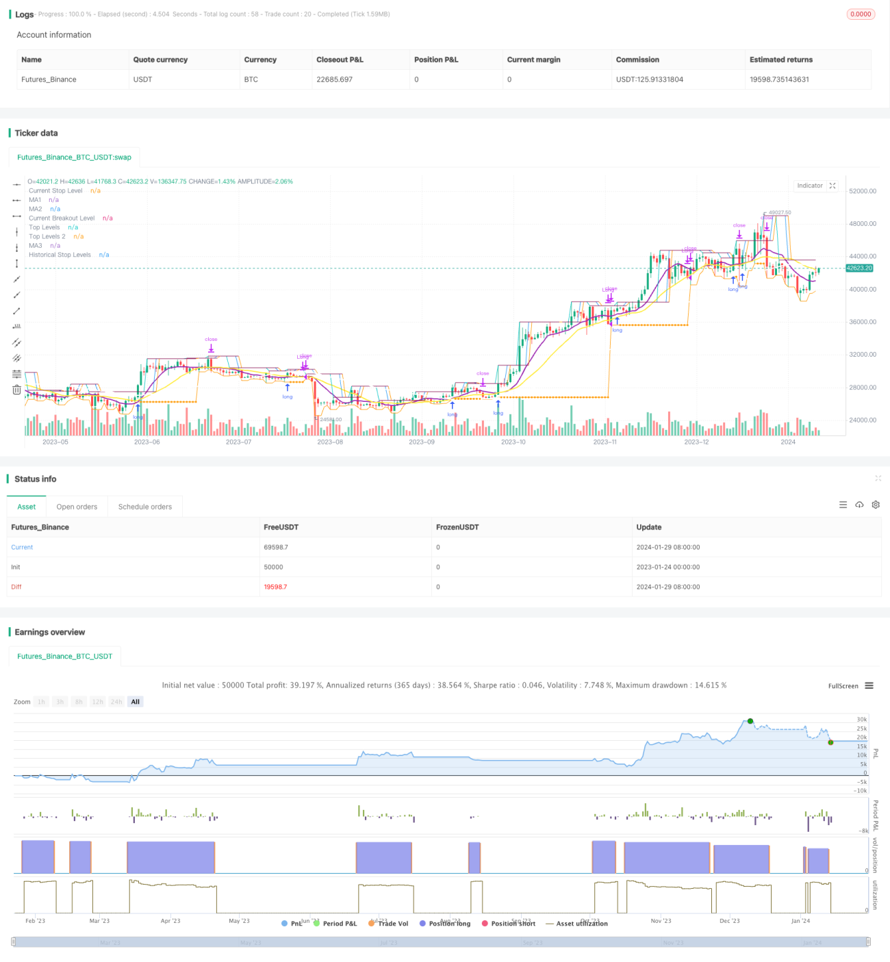
No geral, esta é uma estratégia típica de rastreamento de ruptura. A julgar por quadros de tempo duplos, usando o Swing High para identificar o tempo de entrada e usando a linha de stop loss e mecanismos de saída de seguro de média móvel dupla formam um sistema lógico completo. As características de risco e retorno desta estratégia são claras, adequadas para investidores de rastreamento de médio e longo prazo. Embora existam certos riscos, eles podem ser reduzidos por otimização de parâmetros e regras. A estratégia tem grande espaço para melhoria. Incorporar mais indicadores pode melhorar ainda mais o efeito da estratégia.

/*backtest
start: 2023-01-24 00:00:00
end: 2024-01-30 00:00:00
period: 1d
basePeriod: 1h
exchanges: [{"eid":"Futures_Binance","currency":"BTC_USDT"}]
*/

// This source code is subject to the terms of the Mozilla Public License 2.0 at https://mozilla.org/MPL/2.0/
// © millerrh

// The intent of this strategy is to buy breakouts with a tight stop on smaller timeframes in the direction of the longer term trend.
// Then use a trailing stop of a close below either the 10 MA or 20 MA (user choice) on that larger timeframe as the position 
// moves in your favor (i.e. whenever position price rises above the MA).
// Option of using daily ATR as a measure of finding contracting ranges and ensuring a decent risk/reward.
// (If the difference between the breakout point and your stop level is below a certain % of ATR, it could possibly find those consolidating periods.)

//@version=4
strategy("Qullamaggie Breakout", overlay=true, initial_capital=10000, currency='USD', 
   default_qty_type=strategy.percent_of_equity, default_qty_value=100, commission_type=strategy.commission.percent, commission_value=0.1)
   
// === BACKTEST RANGE ===
Start = input(defval = timestamp("01 Jan 2019 06:00 +0000"), title = "Backtest Start Date", type = input.time)
Finish = input(defval = timestamp("01 Jan 2100 00:00 +0000"), title = "Backtest End Date", type = input.time)

// Inputs
lb = input(defval = 3, title = "Lookback Period for Swing High", minval = 1,
   tooltip = "Lookback period for defining the breakout level.")
lbStop = input(defval = 3, title = "Lookback Bars for Stop Level", minval = 1,
   tooltip = "Initial stop placement is the lowest low this many bars back. Allows for tighter stop placement than referencing swing lows.")  
htf = input(defval="D", title="Timeframe of Moving Averages", type=input.resolution,
  tooltip = "Allows you to set a different time frame for the moving averages. The default behavior is to identify good tightening setups on a larger timeframe
  (like daily) and enter the trade on a breakout occuring on a smaller timeframe, using the moving averages of the larger timeframe to trail your stop.")
maType = input(defval="SMA", options=["EMA", "SMA"], title = "Moving Average Type")
ma1Length = input(defval = 10, title = "1st Moving Average Length", minval = 1)
ma2Length = input(defval = 20, title = "2nd Moving Average Length", minval = 1)
ma3Length = input(defval = 50, title = "3rd Moving Average Length", minval = 1)
useMaFilter = input(title = "Use 3rd Moving Average for Filtering?", type = input.bool, defval = true,
  tooltip = "Signals will be ignored when price is under this slowest moving average.  The intent is to keep you out of bear periods and only
             buying when price is showing strength or trading with the longer term trend.")
trailMaInput = input(defval="2nd Moving Average", options=["1st Moving Average", "2nd Moving Average"], title = "Trailing Stop")

// MA Calculations
ma(maType, src, length) =>
    maType == "EMA" ? ema(src, length) : sma(src, length) //Ternary Operator (if maType equals EMA, then do ema calc, else do sma calc)
ma1 = security(syminfo.tickerid, htf, ma(maType, close, ma1Length))
ma2 = security(syminfo.tickerid, htf, ma(maType, close, ma2Length))
ma3 = security(syminfo.tickerid, htf, ma(maType, close, ma3Length))

plot(ma1, color=color.purple, style=plot.style_line, title="MA1", linewidth=2, transp = 60)
plot(ma2, color=color.yellow, style=plot.style_line, title="MA2", linewidth=2, transp = 60)
plot(ma3, color=color.white, style=plot.style_line, title="MA3", linewidth=2, transp = 60)

// === USE ATR FOR FILTERING ===
// The idea here is that you want to buy in a consolodating range for best risk/reward. So here you can compare the current distance between 
// support/resistance vs.the ATR and make sure you aren't buying at a point that is too extended from normal.
useAtrFilter = input(title = "Use ATR for Filtering?", type = input.bool, defval = false,
  tooltip = "Signals will be ignored if the distance between support and resistance is larger than a user-defined percentage of Daily ATR. 
             This allows the user to ensure they are not buying something that is too extended and instead focus on names that are consolidating more.")
atrPerc = input(defval = 100, title = "% of Daily ATR Value", minval = 1)
atrValue = security(syminfo.tickerid, "D", atr(14))*atrPerc*.01

// === PLOT SWING HIGH/LOW AND MOST RECENT LOW TO USE AS STOP LOSS EXIT POINT ===
// Change these values to adjust the look back and look forward periods for your swing high/low calculations
pvtLenL = lb
pvtLenR = lb

// Get High and Low Pivot Points
pvthi_ = pivothigh(high, pvtLenL, pvtLenR)
pvtlo_ = pivotlow(low, pvtLenL, pvtLenR)

// Force Pivot completion before plotting.
Shunt = 1 //Wait for close before printing pivot? 1 for true 0 for flase
maxLvlLen = 0 //Maximum Extension Length
pvthi = pvthi_[Shunt]
pvtlo = pvtlo_[Shunt]

// Count How many candles for current Pivot Level, If new reset.
counthi = barssince(not na(pvthi))
countlo = barssince(not na(pvtlo))
 
pvthis = fixnan(pvthi)
pvtlos = fixnan(pvtlo)
hipc = change(pvthis) != 0 ? na : color.maroon
lopc = change(pvtlos) != 0 ? na : color.green

// Display Pivot lines
plot((maxLvlLen == 0 or counthi < maxLvlLen) ? pvthis : na, color=hipc, transp=0, linewidth=1, offset=-pvtLenR-Shunt, title="Top Levels")
// plot((maxLvlLen == 0 or countlo < maxLvlLen) ? pvtlos : na, color=lopc, transp=0, linewidth=1, offset=-pvtLenR-Shunt, title="Bottom Levels")
plot((maxLvlLen == 0 or counthi < maxLvlLen) ? pvthis : na, color=hipc, transp=0, linewidth=1, offset=0, title="Top Levels 2")
// plot((maxLvlLen == 0 or countlo < maxLvlLen) ? pvtlos : na, color=lopc, transp=0, linewidth=1, offset=0, title="Bottom Levels 2")

// BUY CONDITIONS
stopLevelCalc = valuewhen(pvtlo_, low[pvtLenR], 0) //Stop Level at Swing Low
buyLevel = valuewhen(pvthi_, high[pvtLenR], 0) //Buy level at Swing High
plot(buyLevel, style=plot.style_line, color=color.blue, title = "Current Breakout Level", show_last=1, linewidth=1, transp=50, trackprice=true)

// Conditions for entry and exit
stopLevel = float(na) // Define stop level here as "na" so that I can reference it in the inPosition 
  // variable and the ATR calculation before the stopLevel is actually defined.
buyConditions = (useMaFilter ? buyLevel > ma3 : true) and
  (useAtrFilter ? (buyLevel - stopLevel[1]) < atrValue : true)
// buySignal = high > buyLevel and buyConditions
buySignal = crossover(high, buyLevel) and buyConditions
trailMa = trailMaInput == "1st Moving Average" ? ma1 : ma2
sellSignal = crossunder(close, trailMa)
// sellSignal = security(syminfo.tickerid, htf, close < trailMa) and security(syminfo.tickerid, htf, close[1] < trailMa)


// STOP AND PRICE LEVELS
inPosition = bool(na)
inPosition := buySignal[1] ? true : sellSignal[1] ? false : low <= stopLevel[1] ? false : inPosition[1]

lowDefine = lowest(low, lbStop)
stopLevel := inPosition ? stopLevel[1] : lowDefine
// plot(stopLevel)

buyPrice = buyLevel
buyPrice := inPosition ? buyPrice[1] : buyLevel
plot(stopLevel, style=plot.style_line, color=color.orange, title = "Current Stop Level", show_last=1, linewidth=1, transp=50, trackprice=true)
plot(inPosition ? stopLevel : na, style=plot.style_circles, color=color.orange, title = "Historical Stop Levels", transp=50, trackprice=false)
// plot(buyPrice, style=plot.style_line, color=color.blue, linewidth=1, transp=50, trackprice=true)

// (STRATEGY ONLY) Comment out for Study
strategy.entry("Long", strategy.long, stop = buyLevel, when = buyConditions)
strategy.exit("Exit Long", from_entry = "Long", stop=stopLevel[1])
if (low[1] > trailMa)
    strategy.close("Long", when = sellSignal)
// if (low[1] > trailMa)
//     strategy.exit("Exit Long", from_entry = "Long", stop=trailMa) //to get this to work right, I need to reference highest highs instead of swing highs
    //because it can have me buy right back in after selling if the stop level is above the last registered swing high point.

Mais.